🔎 Stair step demand and supply curves?

A discrete good is a good where you can’t buy a fraction of a unit. You can buy 1 cell phone or 2 cell phones, but you can’t buy 1.5 cell phones.

In contrast, a continuous good is a good where you can buy a fraction of a unit. You can buy half a gallon of gas or half an ounce of gold. You could even buy your best approximation of 3.1415926 gallons of gas of the same number of ounces of gold.

So far, we’ve focused on continuous goods, and we all know what the demand or supply curve for a continuous good looks like. ↗

This demand curve implies that 1 person has a willingness to pay of $20. Let’s call that person Alice.
If Alice is the person with the highest willingness to pay, there must be another individual with the second highest willingness to pay. Let’s all that person Bob. For simplicity, we’ll assume that there aren’t that many people and that Bob’s willingness to pay is $19

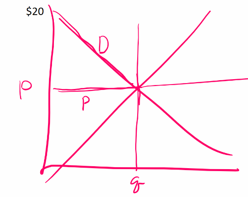
In a Welfare Economics problem, sometimes you will see the demand curve or supply curve for a discrete good. To the left is a demand curves for a discrete good.

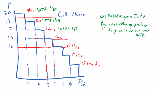
A discrete good is a good that you can’t purchase a fractional quantity of. For example, you can’t purchase half a cell phone or half a laptop.

With a discrete good, it wouldn’t make sense to have standard diagonal D and S curves.

$P = \$19.50 \to Q^D = 1$ (Alice would get a CS of $.50)
$P = \$19.01 \to Q^D = 1$ (Alice would get a CS of $.99)
$P = \$19.99 \to Q^D = 1$ (Alice would get a CS of $.01)
$P = \$20.01 \to Q^D = 0$ (Alice won’t buy, so she has a CS of $0)
$P = \$18.99 \to Q^D = 2$ (Alice and Bob buy. Alice CS=$1.01, Bob’s CS is $.01)

$P = \$17.00 \to Q^D = ?$ ← we don’t have a good answer because Dan is indifferent between purchasing the phone and not purchasing the phone. Specifically, consumers could demand either 3 or 4 phones.

Let’s think about the consumers. At a price of $17, Dan isn’t excited about buying the phone. He’d get a CS of $0
($CS = WTP - P = \$17 - \$17$). From his perspective, he is indifferent between buying it or not buying it. We can’t predict his behavior, because it would be rational either to buy or not buy.

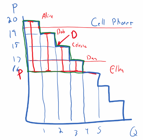
For any given consumer, their personal consumer surplus is their willingness to pay minus the price they actually pay.
$CS = \text{WillingnessToPay} - \text{Price} = WTP - P$

Because we measure the benefit that people receive from a widget by seeing how much they are willing to pay, we can define marginal benefit = willingness to pay. Another way of thinking about it is that CS is the benefit they get from the good minus the price that they pay:
$CS = \text{MarginalBenefit} - \text{Price} = MB - \text{Price}$

Economists generally assume that you can assess the marginal benefit that someone gets from a good by looking at their willingness to pay. For example, given that we assume that Alice is rational, then her willingness to pay up to $20 for a phone implies that her marginal benefit from the phone is at least $20. In contrast, the fact that she’s not willing to pay more than $20, implies that her MB can’t be higher than $20. Based on her behavior, we can very precisely pinpoint her willingness to pay at $20. Therefore, we generally equate MB and WTP.

Willingness to pay can be read from the demand curve. Therefore, we also equate willingness to pay with the demand curve.

In summary,

$\text{Marginal Benefit} = \text{Willingness to Pay} = \text{Demand Curve}$
$MB = WTP = D$

Suppose $P = \$16$

Person	WTP/MB	Consumer Surplus
Alice	$20	$WTP - P = \$20 - \$16 = \$4.00$
Bob	$19	$\$19 - \$16 = \$3$
Celeste	$18	$\$18 - \$16 = \$2$
Dan	$17	$1
Ellen	$16	$0
Total		$4 + 3 + 2 + 1 + 0 = \$10$

Now, let’s assume that the market for Cell Phones is much larger. Here, there are far more steps, so it begins to look like a downward sloping curve.

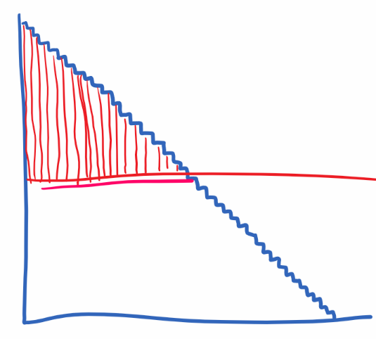
THIS IS WHY WE USE A NICE DOWNWARD SLOPING CURVE FOR DISCRETE GOODS WHEN MANY UNITS ARE BEING SOLD.

Suppose there are millions of cell phones being sold. The downward sloping demand curve basically looks like this.

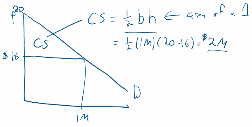
How do we calculate CS now. Previously, we had a way, and everyone here gave me the right answer. It was very intuitive. But how do we do it now, when we use a downward sloping curve to indicate the demand curve.

To find out the area that represents consumer surplus, just imagine the demand curve as being made up of thousands or millions of individual consumers. Draw a line to represent each of their consumer surpluses. If you calculate the area that is filled in with lines, that will be the sum of everyone’s CS, so it will be the society’s CS.

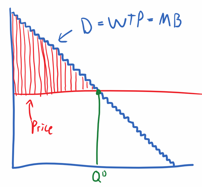
If you do this, you’ll note the following conclusion: Consumer Surplus is the area:

1. below the demand curve
2. above the price line
3. to the left of the Q^D.

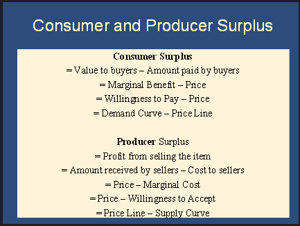
Summary:

Supply

For sellers, their surplus is the profit that they get from selling that unit.
$\text{Profit from selling an additional unit} = \text{Price} - \text{Marginal Cost}$
$= P - MC$
We measure their marginal cost by looking at when they are willing to sell, and we measure that through looking at their supply curve.

Therefore,

$\text{Marginal Cost} = \text{Willingness to Accept} = \text{Supply curve}$
$MC = WTA = S$

Firm	WTA=MC	Producer Surplus
Alpha	$12	$P - WTA = \$16 - \$12 = \$4.00$
Beta	$13	$\$16 - \$13 = \$3$
Charlie	$14	$\$16 - \$14 = \$2$
Delta	$15	$\$16 - \$15 = \$1$
Echo	$16	$P - WTS = \$16 - \$16 = \$0$
Total Profit Producer Surplus		$4 + 3 + 2 + 1 + 0 = \$10$

Between the 5 producers, they are making $10 of profit from selling these units.

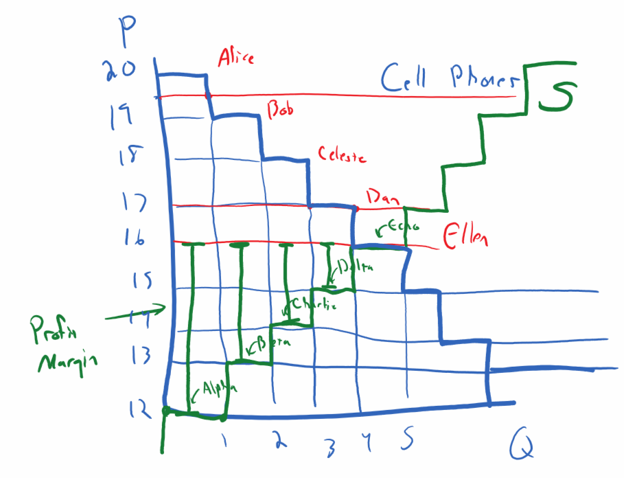
BUT we don’t call it profit because Producer surplus ignores any fixed costs that the firm might have. That’s why we call it producer surplus.