🔎 Long-Run vs. Short-Run Costs (SAC vs LAC vs LMC)

Before we discuss Long-Run vs. Short-Run costs, we should review the concept of the Long-Run vs. Short-Run.

When he covered production functions, he gave the following definitions: (I’ve included some commentary)

• fixed input Production factor that cannot be varied.
• Short Run - Period of time in which quantities of one or more inputs to production cannot be changed.
  • As a result of these fixed inputs, fixed costs are truly fixed in the short run.
• Long Run - Amount of time needed to make all production inputs variable.
  • Because the production inputs are variable, the fixed costs that result from these fixed inputs also become variable. In other words, in the long run, fixed costs generally become variable costs.

Later on, he introduces the following:

• Short-run average cost curve (SAC) - Curve relating average cost of production to output when certain inputs (such as capital) are fixed.
• Long-run average cost curve (LAC) - Curve relating average cost of production to output when all inputs, (including capital) are variable.
• Long-run marginal cost curve (LMC) - Curve showing the change in long-run total cost as output is increased incrementally by 1 unit, in the long run, when all inputs are variable.

In short, we can have different cost curves in the long run, because in the long run we are able to adjust all of the inputs that are fixed in the short run. In general, costs should be lower in the long run than in the short run because of this flexibility.

Note: We will often imagine that it takes time to build a new factory or sell an old factory, but that a firm can hire and/or fire quickly. Therefore, we will often use examples in which capital is a fixed cost and labor is a variable cost. You can adjust this assumption as you apply economic thinking in your own life, be we will often use it as a convention out of habit.

Caveat: When we are talking about perfect competition and monopolistic competition, these fixed inputs can delay entry or exit. For example, if it takes a long time to purchase/build a new factory, then this means that there may be a delay before new firms can enter (or exit) the market. Therefore, for these market structures, we assume that no producers can exit or enter the market in the short run (due to the fixed factors of production). However, in the long run, these fixed factors of production become variable and entry and exit are possible. This why we say that a firm can shut down in the short run, but can’t exit until the long run. If you shut down, you are still paying your lease on your factory. It isn’t until the long run that you can exit this burdensome cost.

🙋I read that the short run is not determined by a specific length of time for example “less than a year” doesn’t necessarily qualify as the definition for the short run.

✔ Yes  ✅

How do these concepts apply to the following diagram?

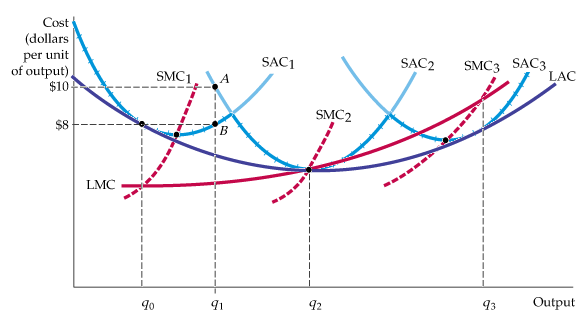
First, I’m going to assume that the only fixed cost is the factory. The factory can be very large, very small, or anything in between - let’s assume that you have very clever architects and engineers, who can come up with wide variety of scales for the factory.

Let’s identify 3 scales:

• Scale 1 is the smallest factory, which is optimized for smaller production runs and can’t do larger production runs. It can only do medium sized production runs at high cost.
• Scale 2 is a medium sized factory, which is optimized for medium production runs. At small scales or large scales, it runs at a higher cost.
• Scale 3 is a larger factory, which is optimized for larger production runs. At small scales it runs at a prohibitively large cost.

If you have factory 1, then, in the short run, you can’t adjust your level of capital. In the short run, you are stuck with that factory. As a result, you AC curve is SAC₁ and your MC curve is SMC₁.

In contrast, if you had factory 2, then in the short run, you still can’t adjust your level of capital (adjust capital = switch the size of your factory). In this case you are stuck with SAC₂ and SMC₂.
Whatever factory you have gives you a different SAC and SMC.

Note that with a medium sized factory, you can have large costs, even if you produce $q = 0$ (the u-shaped blue lines look like they stop, but they go all the way to the y axis. And for the medium and especially the large factory, they get quite large!!). The costs get so large in some cases, that the SAC curve isn’t shown.

The cost curves represent the costs of all inputs that you use, such as your factor, your labor costs, your materials cost and energy costs.

If you have a small factory, you SAC₁ stars relatively low (compared to the expensive factory costs in SAC₂). Your SMC₁ also starts out quite low. You have a small factory that has a great deal of excess capacity. If you want to produce your first unit, the MC of doing is quite low. As you want to produce more and more units, your SMC steadily rises.

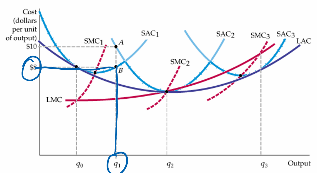
The interesting thing happens when you are producing q₁. At q₁, if you happen to have factory 1, then your average costs are $8. In the short run, if you happen to have factory 2, then your average costs are $10.

How about in the long run? Let’s assume that there are only the three factory size that we discussed above. Suppose you start with the medium factory. What will your costs be in the long run if you know that you will always be producing q₁ units. In the short run, your costs will be $10, but in the long run, you will adjust your level of capital and replace your medium factory with a small factory. As a result, while your short run cost, based on the medium factory, is $10, you long run cost, based on the smaller factory is $8.

This explains why we have both a LAC curve and a SAC curve. When you have more time to adjust, you can optimize all of your production inputs (capital, labor, etc.) to their optimal levels and achieve a lower average cost ($8 instead of $10).

🙋 We had 9 production lines running, making 10,000 units per day. Then the great financial crisis happened, and demand contracted, and we found that we had a factory like factory #3. This was a big problem. It was a painful process to downsize to factory from factory #3 to a factory more like factory #1 or factory #2.

✏️ Based on the assumption that there is only three factory sizes, what is the LAC. (Hint: it’s not the LAC from the diagram, because the diagram assumes that you have the clever engineers that can come up with an infinite variety of factory sizes.)

✔ Click here to view answer

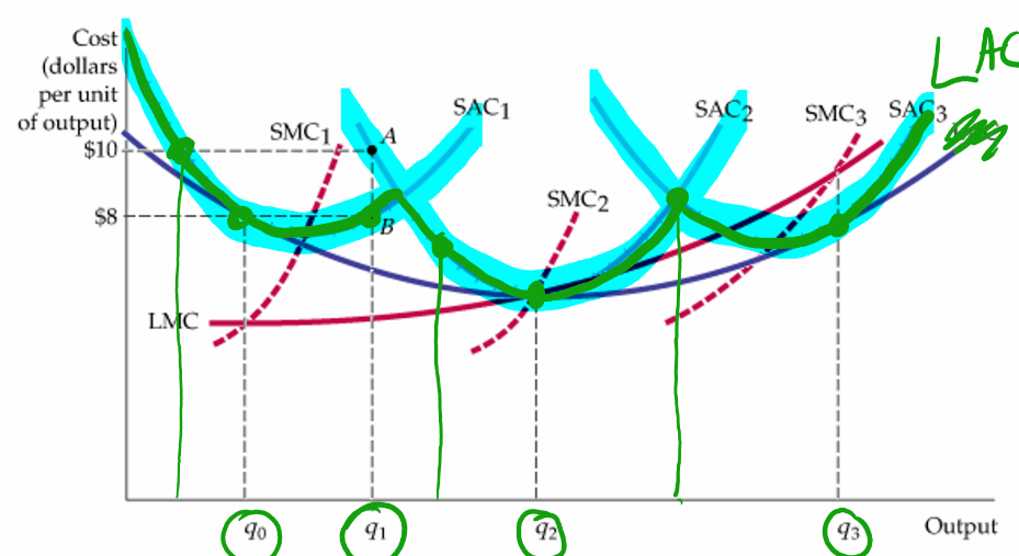
The long-run average cost curve LAC is the green line, known as the “envelope” of the short-run average cost curves SAC1, SAC2, and SAC3. (The envelope means that you take the lowest points on each of the SAC curves to get a curve that is below or on all of the SAC curves.) With economies and diseconomies of scale, the minimum points of the short-run average cost curves do not lie on the long-run average cost curve.  ✅

What if we had more possible factory sizes?

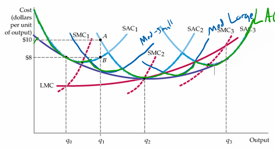
The new green line is the envelope of the FIVE possible factory sizes. The managers will always choose the optimal factory size.

What if there were an infinite number of possible factory sizes?!?! (ie and infinite number of possible SAC curves)
This will cause the smoothing effect of the original line.

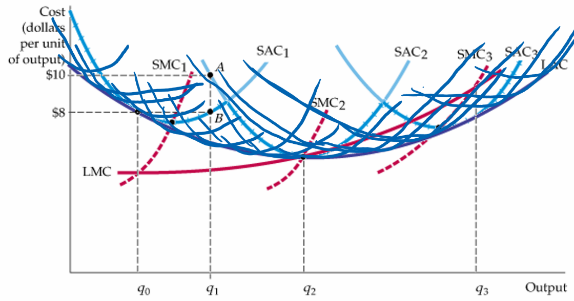
Given the profit motive, for any given quantity that they decide to sell, the engineers will always choose the optimal size for the factory. This results in a relatively smooth LAC curve. (ie. the purple line).

In other words, the LAC is the lower envelope of all of the possible SAC curves that the engineers can come up with.

There is always only one LAC, because it involves the optimal choice of SAC. (optimal = lowest for the quantity I want to produce).

Based on choosing the optimal factory size, you can also calculate the long run marginal cost curve. The Long run Marginal cost curve just tells you how much it costs to make an additional unit of the good if you have time to adjust your factory size.

Short run marginal cost - how much it costs to another pint of pulled pork if you are stuck with your current commercial kitchen (this is relevant for short run planning when you are stuck with your current lease).
Long run marginal cost - how much it costs to make another pint of pulled pork if you have enough time to switch to the optimal size of commercial kitchen (this is relevant for long run planning).

To me, all of the SAC curves in the above diagram look like scalloped potatoes. The scalloped potatoes have a much smaller shape than the dish, but together they match the shape of the enclosing dish. This is similar to how all of the SAC curves make up the shape of the LAC curve.