🔎 Formulas

Formulas will be added to this page as they are covered in class. The formulas are grouped by lecture, and each lecture has a link to the relevant lecture notes.

Press Ctrl-D to bookmark this page. A downloadable paper/Microsoft Word formula sheet can be found in my File Share.

Questions or comments? Please email munger.e1010@gmail.com. Remember, your first reference is always the lectures and the homework. Feel free to download my materials, but please do not reupload them.

Formulas will be added to this document after Bruce has introduced them in class.

L1 - Introduction

Determinants of Market Demand Price Income (Normal vs Inferior, below) Price of Related Goods (Substitutes vs Compliments, below) Tastes and Preferences Expectations Number of Buyers	Determinants of Market Supply Price Input Prices Technology Expectations Number of Sellers

• Normal goods: Goods whose demand increases when income increases
• Inferior goods: Goods whose demand decreases when income increases
• Substitutes: Demand goes up when the price of a substitute goes up
• Complements: Demand goes down when the price of a complement goes up

References: 1 Jan 26.ppt and L1-Introduction

L2 - BC, IC, and Optimization

$$MU_{X} = \frac{\mathrm{\Delta}U}{\mathrm{\Delta}X}$$

Principles of Indifference Curves

• Higher indifference curves represent higher utility
• Indifference curves never cross
• Indifference curves usually slope downward
• Indifference curves are usually convex—bowed inward toward the origin (sometimes called “concave up”)

$\text{Slope of BC} = - \frac{P_X}{P_Y}$
$\text{Slope of IC} = \frac{\Delta Y}{\Delta X} \text{ along IC} = - MRS$
$MRS = \frac{MU_{X}}{MU_{Y}}$

First Condition for a Consumer Optimum:  a) Your optimal consumption bundle (X*,Y*) should be on the Budget Constraint. In other words, you must use all of your money. Alternate Version:  b) $X^∗×P_X +Y^∗×P_Y = B$

Second Condition for a Consumer Optimum:  a) Slope of IC = Slope of BC  b) $\frac{MU_x}{P_x} = \frac{MU_y}{P_y}$ ("Bang for the buck" formulation) This ensures that you spend your money on the things that bring you the most utility per dollar. Alternate versions:  c) $MRS=\frac{P_x}{P_y}$  d) Ratio of MUs: $\frac{MU_x}{MU_y}=\frac{P_x}{P_y}$

References: 2 Feb 2.ppt and L2-Consumer Choice 1

L3 - SE, IE, Demand, and Giffen

I suggest memorizing these by using these rules to replicate the examples Bruce has in the slides and I have on my website. Practice!

Substitution effect: (about relative prices)

1. When one price changes, suddenly one good becomes relatively more expensive and the other becomes relatively cheaper.
2. For the good that is relatively cheaper, you will buy more, so SE↑. For the good that is more expensive, you will buy less, so SE↓.

Income Effect: (about feeling richer or poorer)

1. When a price changes, your purchasing power increases or decreases. Decide which. (If Price↓, purchasing power increases [you feel Richer]. If Price↑, purchasing power decreases [you feel Poorer].)
2. Review the following table

	Richer	Poorer
Normal	IE↑	IE↓
Inferior	IE↓	IE↑

Combined Effect: $CE=IE + SE$. You just add them up.

• ↓ + ↓ = ↓
• ↑ + ↑ = ↑
• If the two effects go in different directions, then “the bigger one wins” (If the question tells you that they buy more then you know that CE↑ - and vice versa.)

Giffen Goods = demand curve slopes upward = when the price increases, you buy more.

• Demand curve downward for normal goods and for non-Giffen inferior goods.
• All Giffen Goods are Inferior Goods BUT Not All Inferior Goods are Giffen Goods.
• For a good to be Giffen: (1) It must be an inferior good and (2) IE must outweigh SE

References: 3 Feb 9.ppt and L3-Consumer Choice 2

L4 - Risk and Insurance

Expected Value (EV)
= Prob of Outcome 1 × Value of Outcome 1
+ Prob of Outcome 2 × Value of Outcome 2
+ Prob of Outcome 3 × Value of Outcome 3
+ …
+ Prob of Outcome N × Value of Outcome N

Expected Utility (EU)
= Prob of Outcome 1 × Utility from Outcome 1
+ Prob of Outcome 2 × Utility from Outcome 2
+ Prob of Outcome 3 × Utility from Outcome 3
+ …
+ Prob of Outcome N × Utility from Outcome N

EV is used to measure the cost of providing insurance. EU is to measure what people will choose.
Marginal utility of money = slope of “utility of money” curve

Risk Aversion ⇨ Diminishing Marginal Utility of Money ⇨ Diminishing Slope of Utility Curve (gets flatter)	Risk Neutrality ⇨ Constant Marginal Utility of Money ⇨ Constant Slope of Utility curve (straight)	Risk Loving ⇨ Increasing Marginal Utility of Money ⇨ Increasing Slope of Utility Curve (gets steeper)
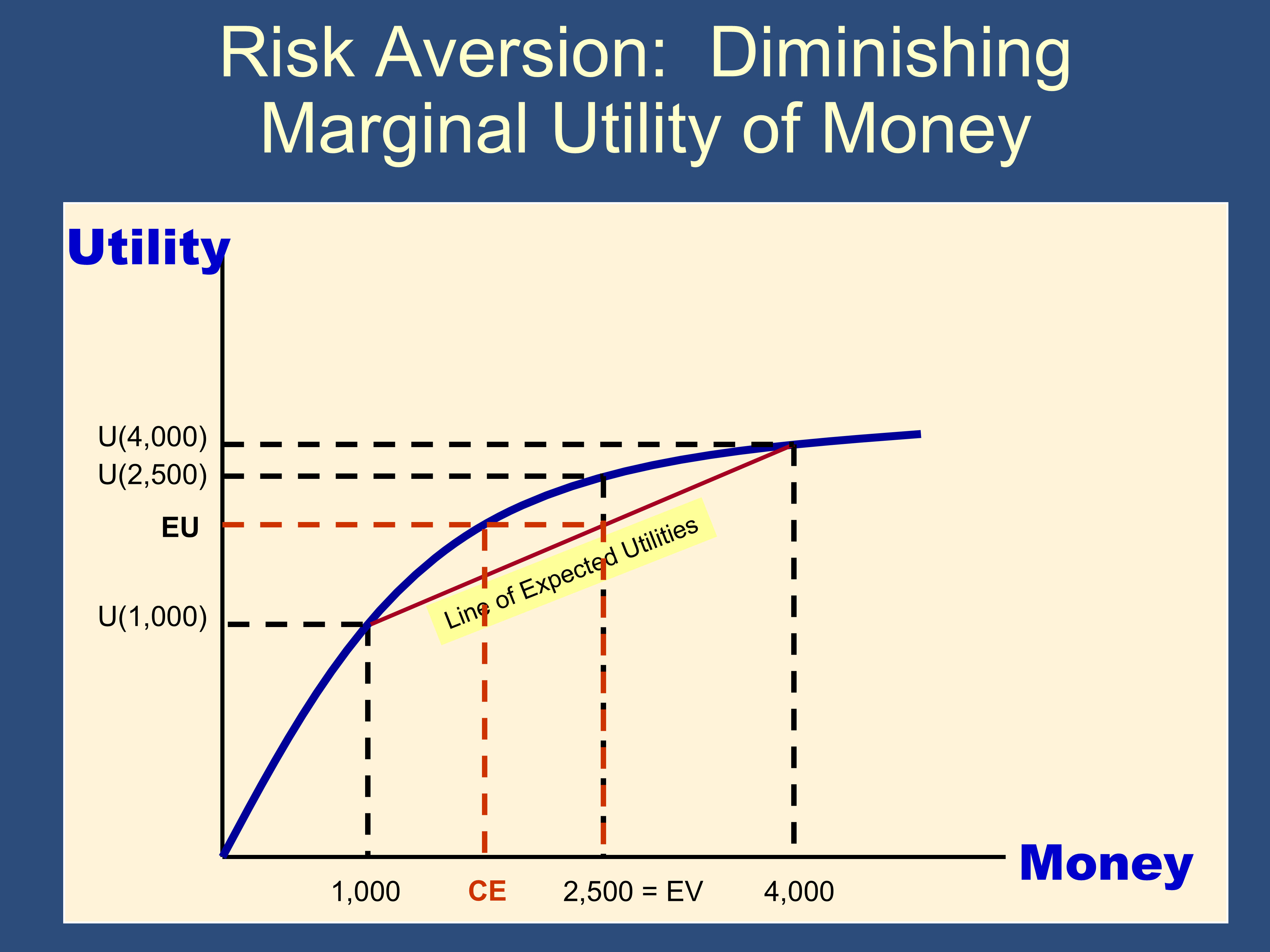Risk Averse: CE < EV	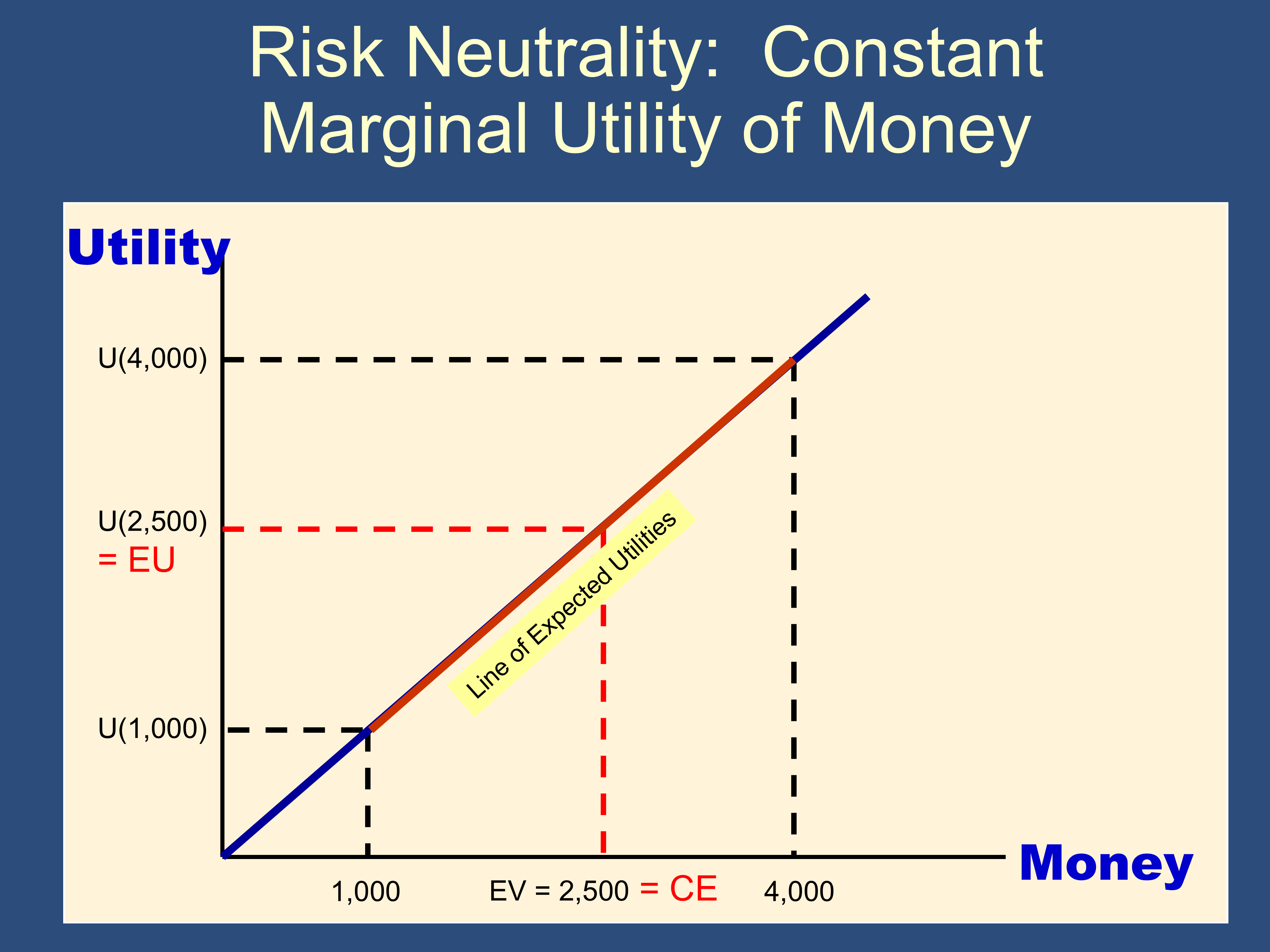Risk Neutral: CE = EV	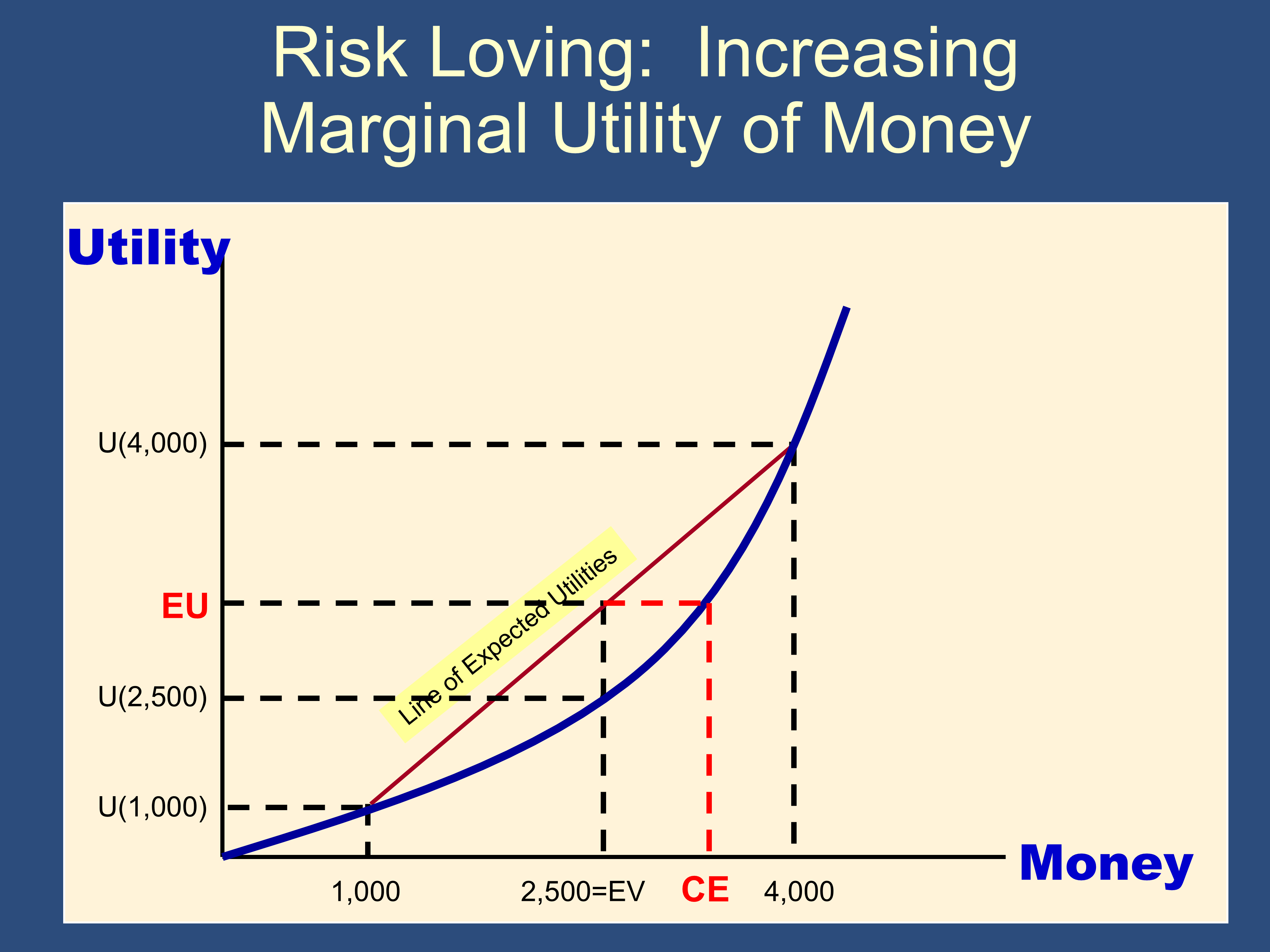Risk Loving: CE > EV

References: 4 Feb 23.ppt and L4-Notes

L5 - Production and Costs

Production

• Returns to Scale: What happens to output when all inputs are changed … … By the same proportion, simultaneously
• Marginal product: What happens to output when one input is changed … … By itself, Holding all other inputs constant
• Average Product: Output per unit of a particular input.
  • Example: average product of labor $= \frac{q}{L}$
• Marginal Product: Additional output produced from one additional unit of an input.
  • Example: marginal product of labor $= \frac{\Delta q}{\Delta L}$

Constant/Increasing/Decreasing Returns to Scale

• Constant Returns to Scale: Increasing all inputs by the same proportion increases output by the same proportion.
  • Example: When all inputs are doubled, output exactly doubles.
• Increasing Returns to Scale: Increasing all inputs by the same proportion increases output by a greater proportion
  • Example: When all inputs are doubled, output more than doubles.
• Decreasing Returns to Scale: Increasing all inputs by the same proportion increases output by a smaller proportion
  • Example: When all inputs are doubled, output increases by less than double

	Total	Fixed	Variable
Total	$TC$	$TFC$ = costs that do not vary with $q$	$TVC$ = costs that do vary with $q$
Average	$AC = \frac{TC}{q}$	$AFC = \frac{TFC}{q}$	$AVC = \frac{TVC}{q}$
Marginal	$MC = \frac{\Delta TC}{\Delta q}$	$MFC = \frac{\Delta TFC}{\Delta q} = 0$	$MVC = \frac{\Delta TVC}{\Delta q} = MC$

$$TC = TFC + TVC$$ $$AC = AFC + AVC$$ $$MC = 0 + MVC$$

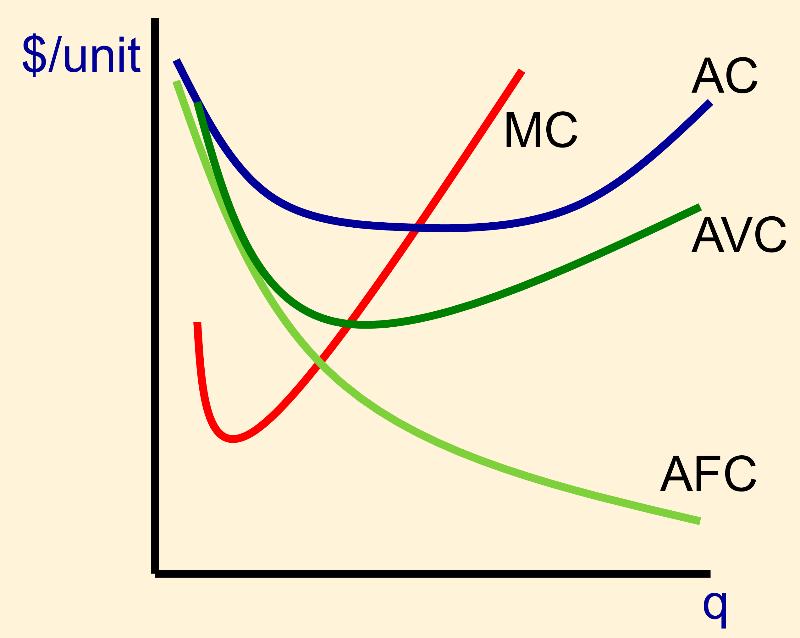
Short Run: Period of time in which quantities of one or more inputs to production cannot be changed.

• Short-run Costs—costs when only one input is allowed to increase as output increases

Long Run: Amount of time needed to make all production inputs variable.

• Long-run Costs—costs when all inputs are allowed to vary as output increases

1. Short-run average Cost curve (SAC): Curve relating average cost of production to output when level of capital is fixed.
2. Long-run Average Cost curve (LAC): Curve relating average cost of production to output when all inputs, including capital, are variable.
3. Long-run Marginal Cost curve (LMC): Curve showing the change in long-run total cost as output is increased incrementally by 1 unit.

Economies of Scale—a given percentage increase in output causes a smaller percentage increase in costs.

• If economies of scale are present, long-run average costs (LAC) will be decreasing

Diseconomies of Scale—a given percentage increase in output causes a larger percentage increase in costs

• If diseconomies of scale are present, long-run average costs (LAC) will be increasing

Economies of Scope: Situation in which joint output of a single firm is greater than output that could be achieved by two different firms when each produces a single product.

Degree of Economies of Scope (SC): Percentage of cost savings resulting when two or more products are produced jointly rather than Individually.

$$SC = \frac{C\left( q_{1} \right) + C\left( q_{2} \right) - C\left( q_{1},q_{2} \right)}{C\left( q_{1},q_{2} \right)}$$

SC > 0 ⇨ economies of scope are present
SC < 0 ⇨ dis economies of scope are present

References: 5 Mar 2.ppt and 5 - Notes

Post Midterm

Sidebar: Comparison of Market Structures

(This section summarizes information from lectures 6-8.)

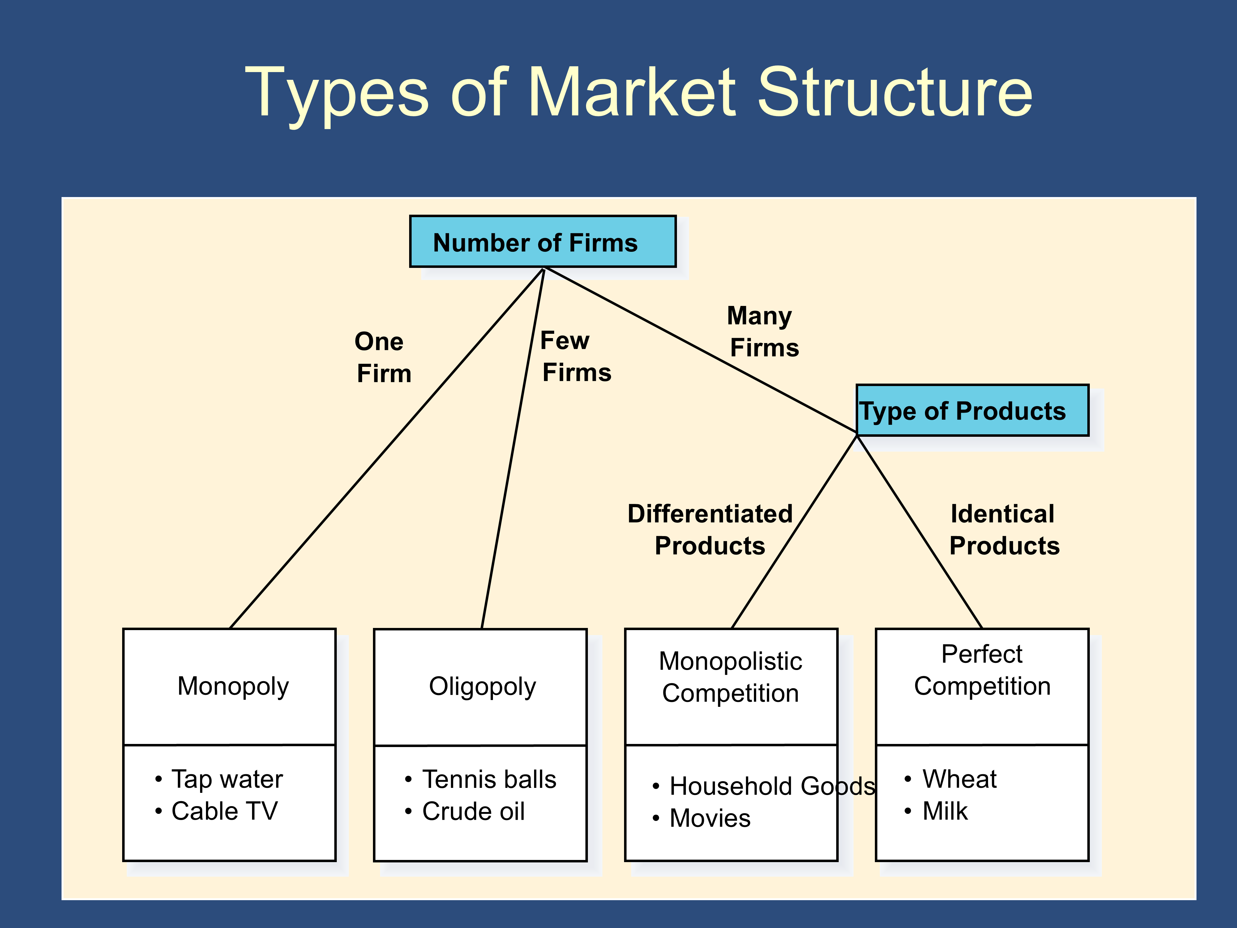
	Perfect Competition	Monopolistic Competition	Monopoly	Oligopoly (I added this column)
Number of Firms	Very many	Many	One	Few
Output of Different Firms	Identical	Differentiated	---	Identical or Differentiated
View of Pricing	Price taker	Price maker	Price maker	Depends
Barriers to Entry/Exit	No	No	Yes	Yes
Output and Pricing	MR = MC = P q* at min AC	MR = MC P > MC q* below min AC	MR = MC P > MC q* below min AC	Use Game Theory
SR Profit	Positive, zero, or negative	Positive, zero, or negative	Positive, zero, or negative	Positive, zero, or negative
LR Profit	Zero	Zero	Positive or Zero	Positive or Zero
Advertising	Never	Always	Sometimes (PR Type)	Depends

L6 - Perfect Competition

TR = p × q = $3 × 1000gal = $3000
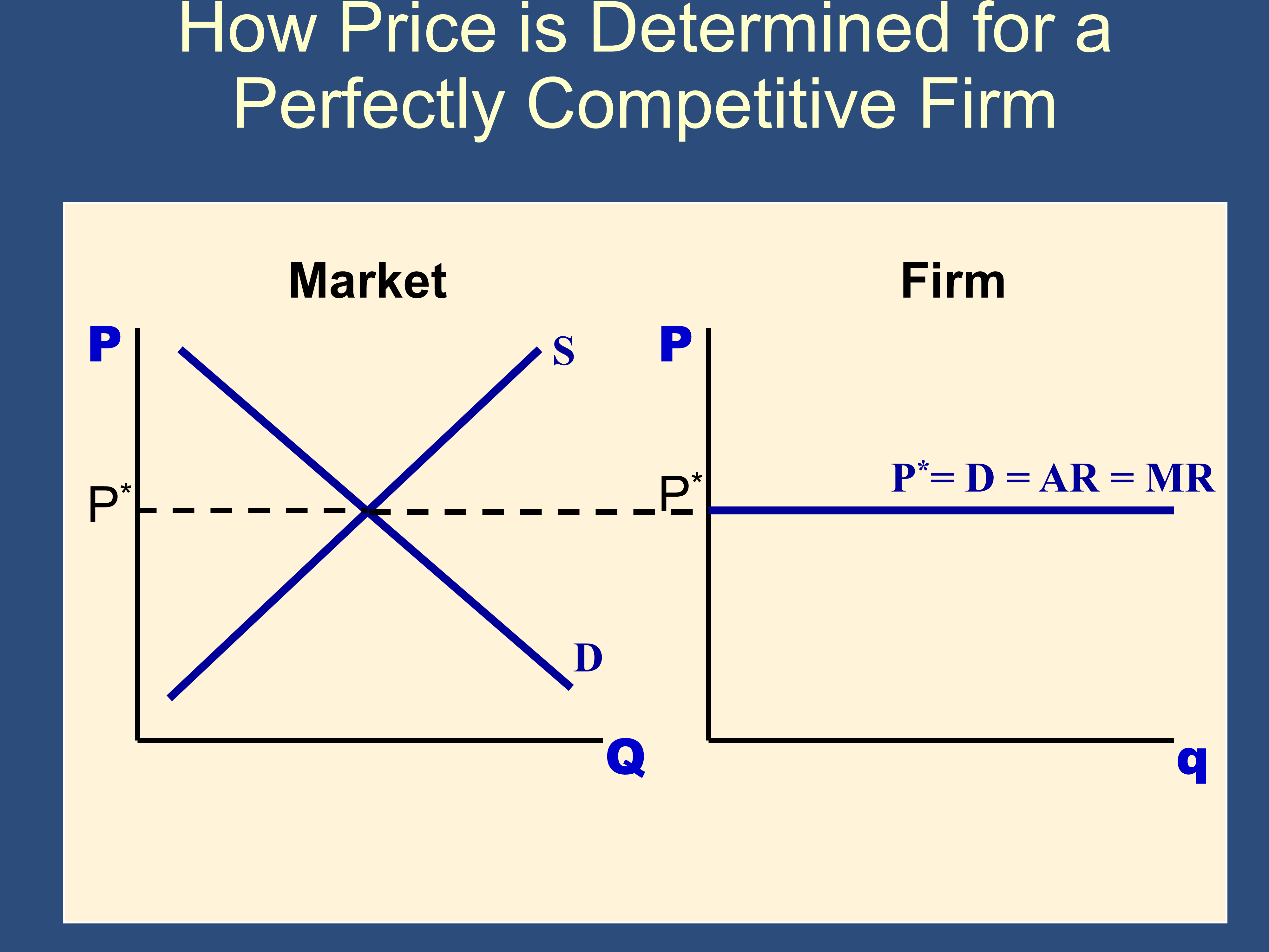
AR = TR/q = p = $3,000/1000gal = $3
MR =∆TR/ ∆q = ($3,003 - $3,000)/(1001 - 1000) = $3 (P=MR in competitive mkts)

Conditions of Perfect Comp:

• Many buyers and sellers
• Complete information
• Well-specified property rights
• Homogeneous products
• Ease of entry and exit
• Price-taking behavior

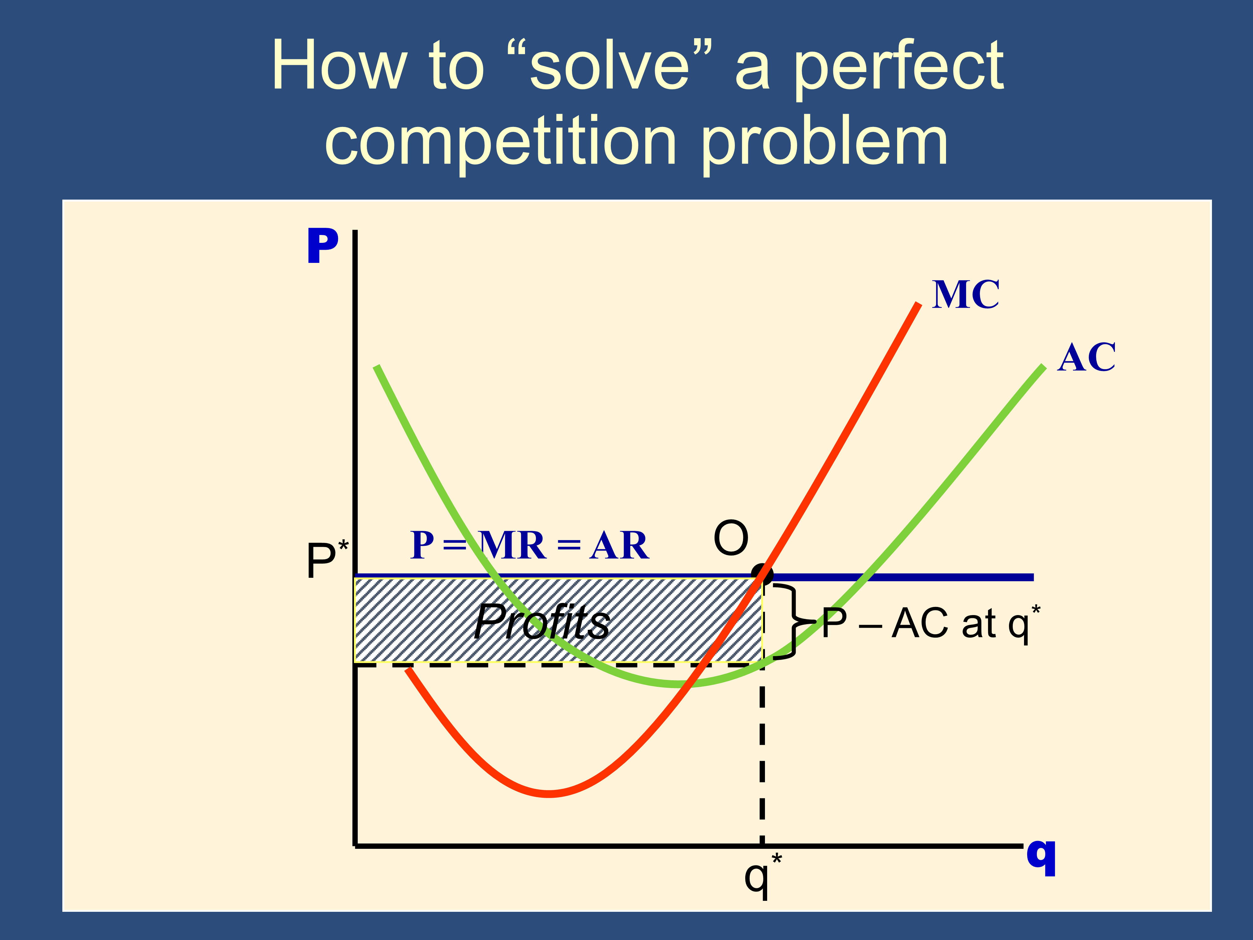
Profit = π = TR - TC = q (p - AC)
(Per-unit profit is P-AC. If P>AC, profit will be positive.)

Profit Maximization Condition:

• For continuous quantities, produce that q for which MR = MC (derived from calculus)
• For discrete quantities, produce the highest q for which MR ≥ MC

Shut down if profits from shutting down > profits from producing q*, ie if AVC>P

How to “solve” a perfect competition problem:
1.) P=MC to figure out q*
2.) Do you shut down (P<AVC) or, in LR, exit (P<ATC)
3.) Wrap up

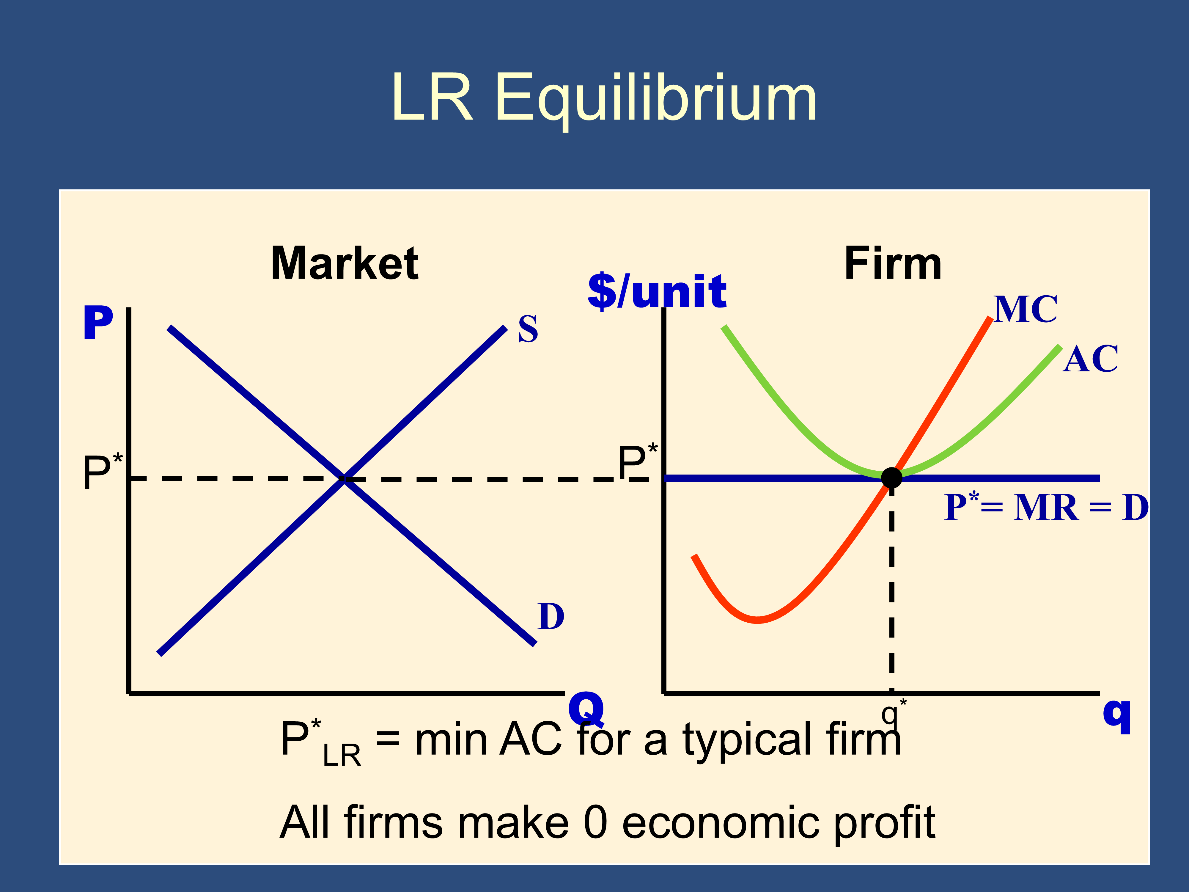
Perfect Competition, Long Run

Accounting Costs = Explicit Costs
Economic Costs = Explicit Costs (ie. Accounting Costs) + Implicit Costs.

Accounting profit = TR – Accounting Costs
Economic Profit = TR – Economic Costs = TR – Explicit Costs – Implicit Costs
In this class, we typically use Economic costs and profit.

Why profit tends to zero in competitive markets:
If π > 0 → Entry occurs → Number of firms ↑ → Supply ↑ → Supply curve shifts R → P*↓, Q*↑, π↓ to 0
If π < 0 → Exit occurs → Number of firms ↓ → Supply ↓ → Supply curve shifts L → P*↑, Q*↓, π↑ to 0

References: 6 Mar 23.ppt and 6 - Notes

L7 - Monopoly

Conditions of Monopoly:

1. One Seller
2. Barriers to Entry

Sources of Monopoly:

• Govt grant of a monopoly
  • Public franchise (A government designation that a firm is the only legal provider of a good or service)
  • Patents and copyrights
• Sole ownership of a scarce resource
• Network externality - when usefulness of a product increases with the number of consumers (Facebook, Uber, Windows)
• Natural monopoly - A natural monopoly occurs when economies of scale are so large that one firm can supply the entire market at a lower average total cost than can two or more firms

In perfect competition, MR = P, but in monopoly, MR < P:

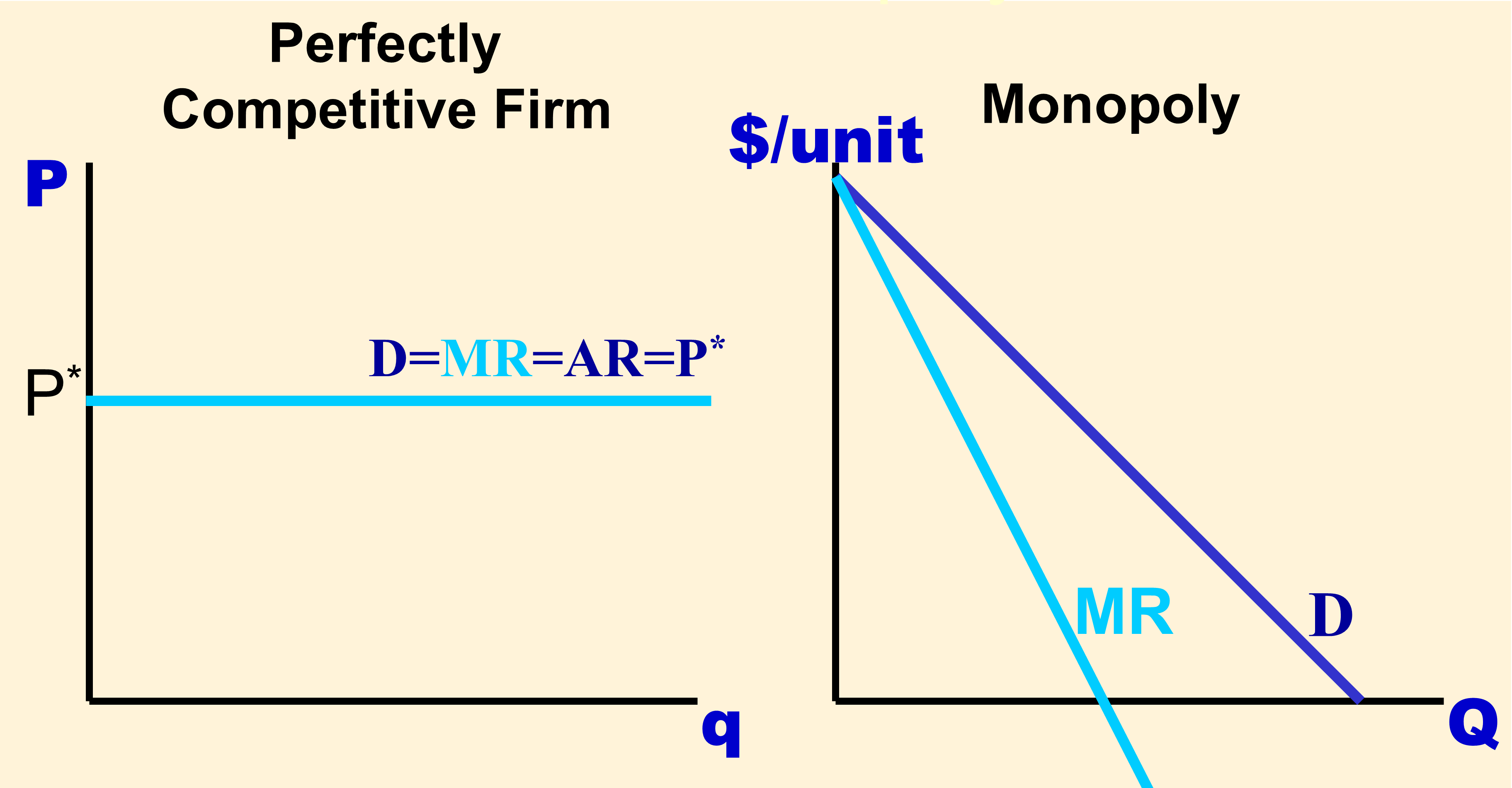
Lerner Index = $`\frac{P - MC}{P}`$ (P-MC is the markup, so the Lerner index measures the markup as a percentage of price.)

$$\frac{P - MC}{P} = - \frac{1}{E_{d}}$$

Price Discrimination - Practice of charging different prices to different consumers for the same or similar goods.

• First-degree (or Perfect) Price Discrimination - Charging each customer her reservation price. (Reservation Price = Maximum price that a customer is willing to pay for a good.)
• Second-degree Price Discrimination - Charging different prices per unit for different quantities of the same good or service.
  • block pricing – Charging different prices for different quantities or “blocks” of a good.
• third-degree price discrimination - Practice of dividing consumers into two or more groups with separate demand curves and charging different prices to each group. Examples: senior or student discounts.

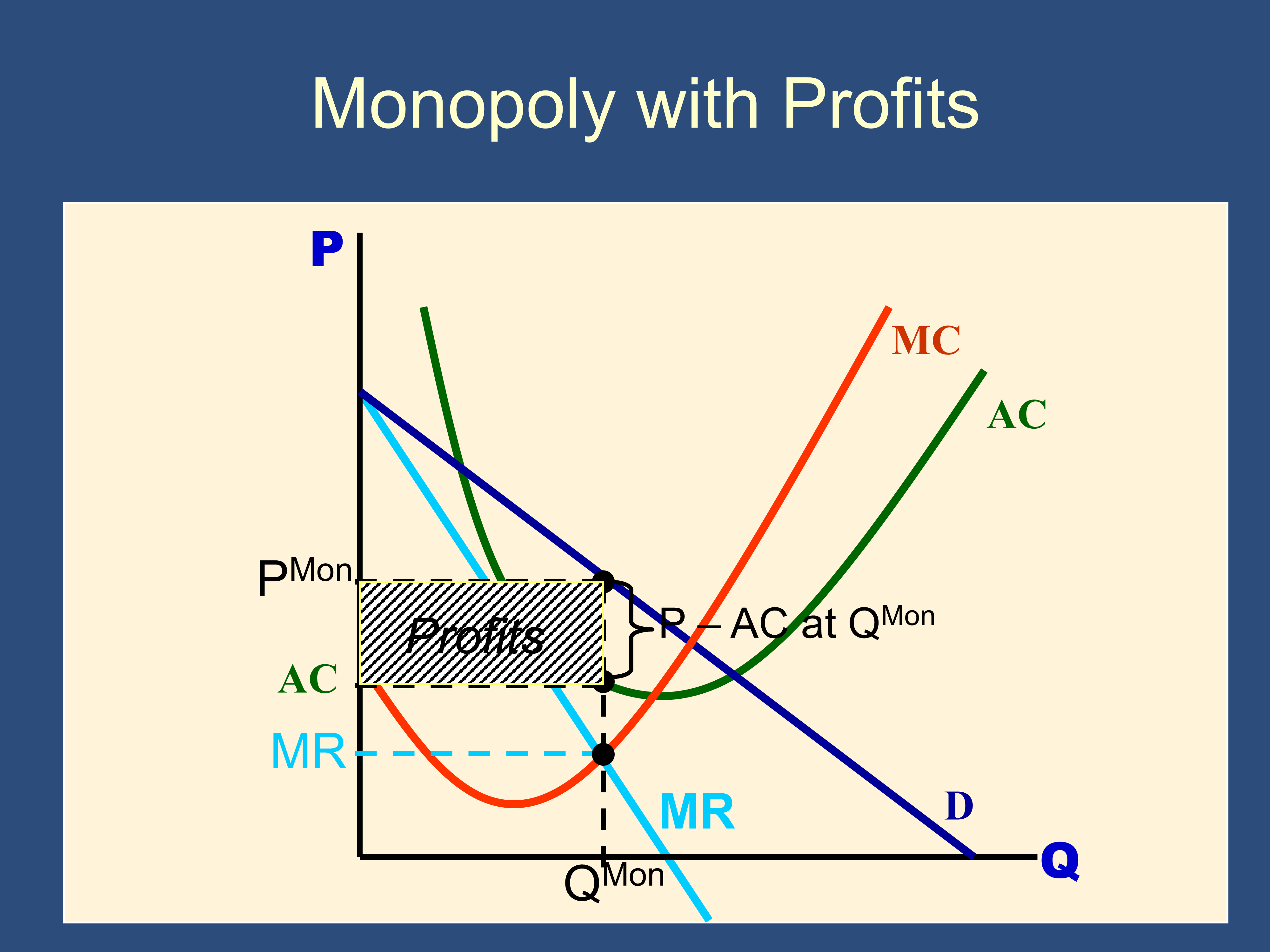
How to “solve” a Monopoly problem

1.) MR=MC to figure out Q
2.) Draw a line up to the demand curve to figure out P
3.) Wrap up. Profit = TR-TC = q*(P-AC)

Monopoly, Short Run and Long Run (with profits)

References: 7 Mar 30.ppt and 7 - Notes

L8a - Monopolistic Competition

Conditions of Monopolistic Competition:

1. Firms compete by selling differentiated products that are substitutes for each other but not perfect substitutes. In other words, the cross-price elasticities of demand are large but not infinite.
2. There is free entry and exit: It is relatively easy for new firms to enter the market with their own brands and for existing firms to leave if their products become unprofitable.

IE:

• Many sellers (like perfect competition)
• Free entry and exit (like perfect competition)
• Downward sloping demand curve (like monopoly)
• Product differentiation (Unlike perfect competition)
• Demand curve much more elastic than monopoly

Sidebar:
Cross-price elasticity of demand - measures the response of demand for one good to changes in the price of another good.

$$Cross - price\ elast.\ of\ D = \frac{\%\ change\ in\ Q^{d}\ for\ good\ 1}{\%\ change\ in\ price\ of\ good\ 2}$$

• For substitutes, cross-price elasticity > 0
  (e.g., an increase in price of Diet Pepsi causes an increase in demand for Diet Coke)
• For perfect substitutes, cross-price elasticity → ∞
• For close (but not perfect) substitutes, cross-price elasticity is high but not infinite

Why profit tends to zero in monopolistic competition markets:

• π > 0 → Entry occurs → Number of firms ↑ → Demand for product of incumbent firms ↓ → Demand curve of incumbent firms shifts left and becomes more elastic → q^MC goes down to point where P = AC → Economic profits are 0
• π < 0 → Exit occurs → Number of firms ↓ → Demand for product of remaining firms ↑ → Demand curve of incumbent firms shifts right and becomes less elastic → q^MC goes up to point where P = AC → Economic profits are 0

In the long run, the market gravitates toward the following. You can see in the following that profit is zero because when the firm produces q^MC, P^MC=AC, so per-unit profit = P-AC = 0.

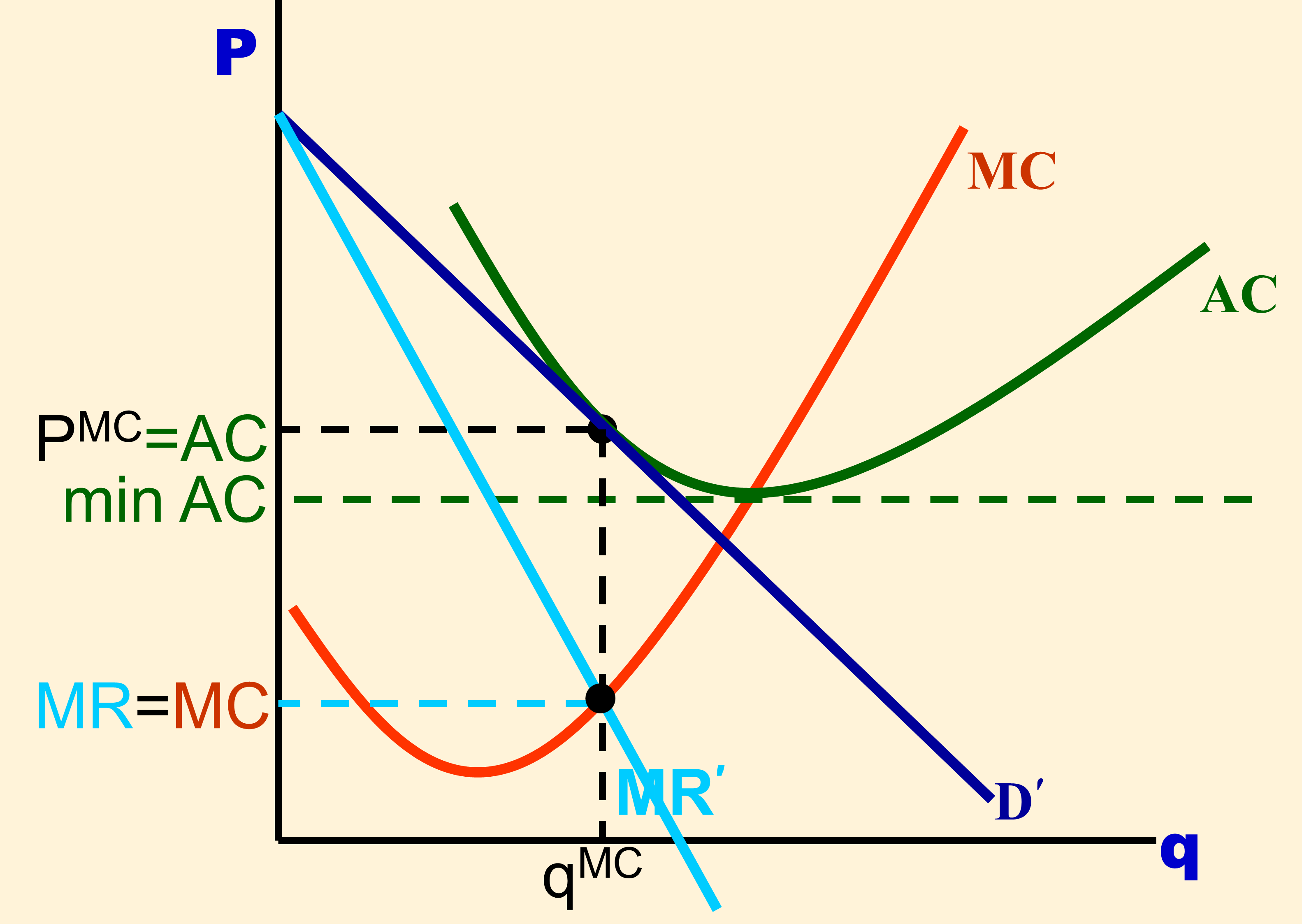
How to “solve” a monopolistic competition problem:

Solve Monopolistic Competition just like Monopoly, except that in the long run, the demand curve shifts until it is tangent to AC and P=AC.

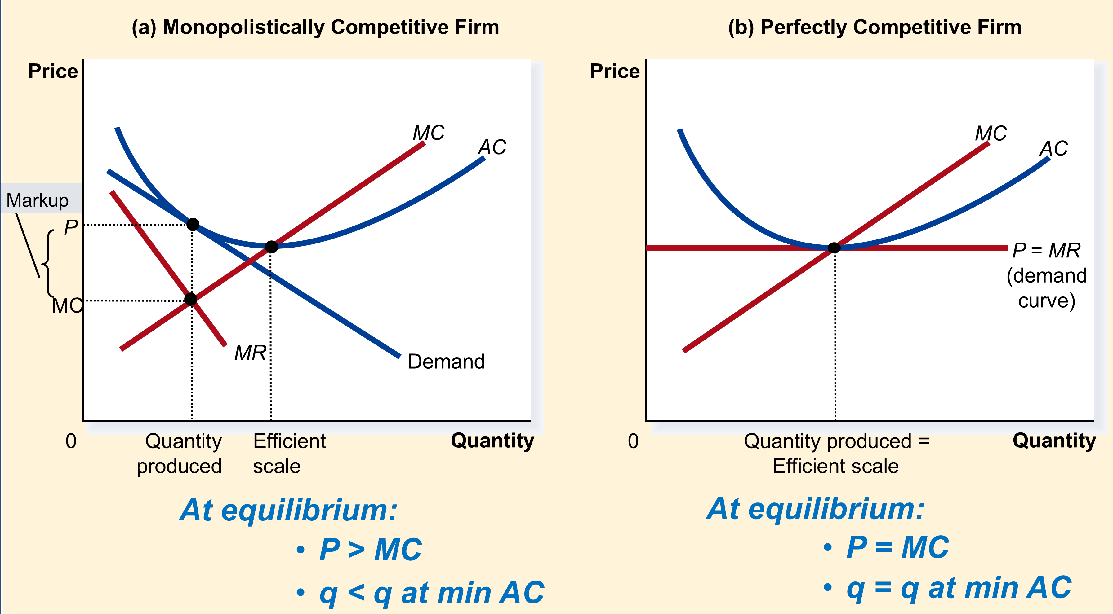
Productive efficiency refers to producing items at the lowest possible cost, i.e. at minimum average cost.
Allocative efficiency refers to producing all goods up to the point where the marginal benefit to consumers is just equal to the marginal cost to firms.
Monopolistic competition results in neither productive nor allocative efficiency.

The perfectly competitive firm is both allocatively efficient and productively efficient.

References: 8a Apr 6.ppt and 8a - Notes

L8b - Oligopoly

Oligopoly: a market structure in which only a few sellers offer homogeneous or differentiated products.
Homogeneous products—goods which are identical or almost perfect substitutes: Steel, Oil, Gasoline, etc.
Strategic behavior in oligopoly: A firm’s decisions can affect other firms and cause them to react. The firm will consider these reactions when making decisions—strategic interdependence Oligopolies typically have barriers to entry like monopolies do.

Four-firm concentration ratio: the percentage of the market’s total output supplied by its four largest firms.
Oligopoly = high concentration ratio = less competition.

Examples of strategic actions by incumbent firms: s

• ***Preemptive investment—***Get there first
• Excess capacity q > q which maximizes profit (p < p consistent with profit maximization)

Nash Equilibrium: Each firm is doing the best it can given what its competitors are doing. (In other words, each competitor is playing a best response to the other competitors.)

Role play each player and consider each action your opponent might take. Highlight or underline your best response .

		Pepsi’s Spending On Advertising
		Small	Large
Coke’s Spending on Advertising	Small	πC = +8 πP = +8	πC = −2 πP = +13
	Large	πC= +13 πP = −2	πC = +3 πP = +3

Two highlights in the same cell means both players are playing a best response. Therefore it is a Nash Equilibrium.
A full row of highlights for the row player means that that row is a dominant strategy. Similarly for the column player.

prisoner’s dilemma: a game in which pursuing dominant strategies results in noncooperation that leaves everyone worse off.

• For example, in the game above, both players have dominant strategies to do large advertising. However, they are worse off if they do this than if they both did small advertising.

Collusion means choosing the cooperative outcome (with the highest combined score). It typically implies doing so in an illegal or unethical manner.

repeated game Game in which actions are taken and payoffs received over and over again.
tit-for-tat strategy Repeated-game strategy in which a player responds in kind to an opponent’s previous play, cooperating with cooperative opponents and retaliating against uncooperative ones.

References: 8b Apr 6.ppt and 8b - Notes

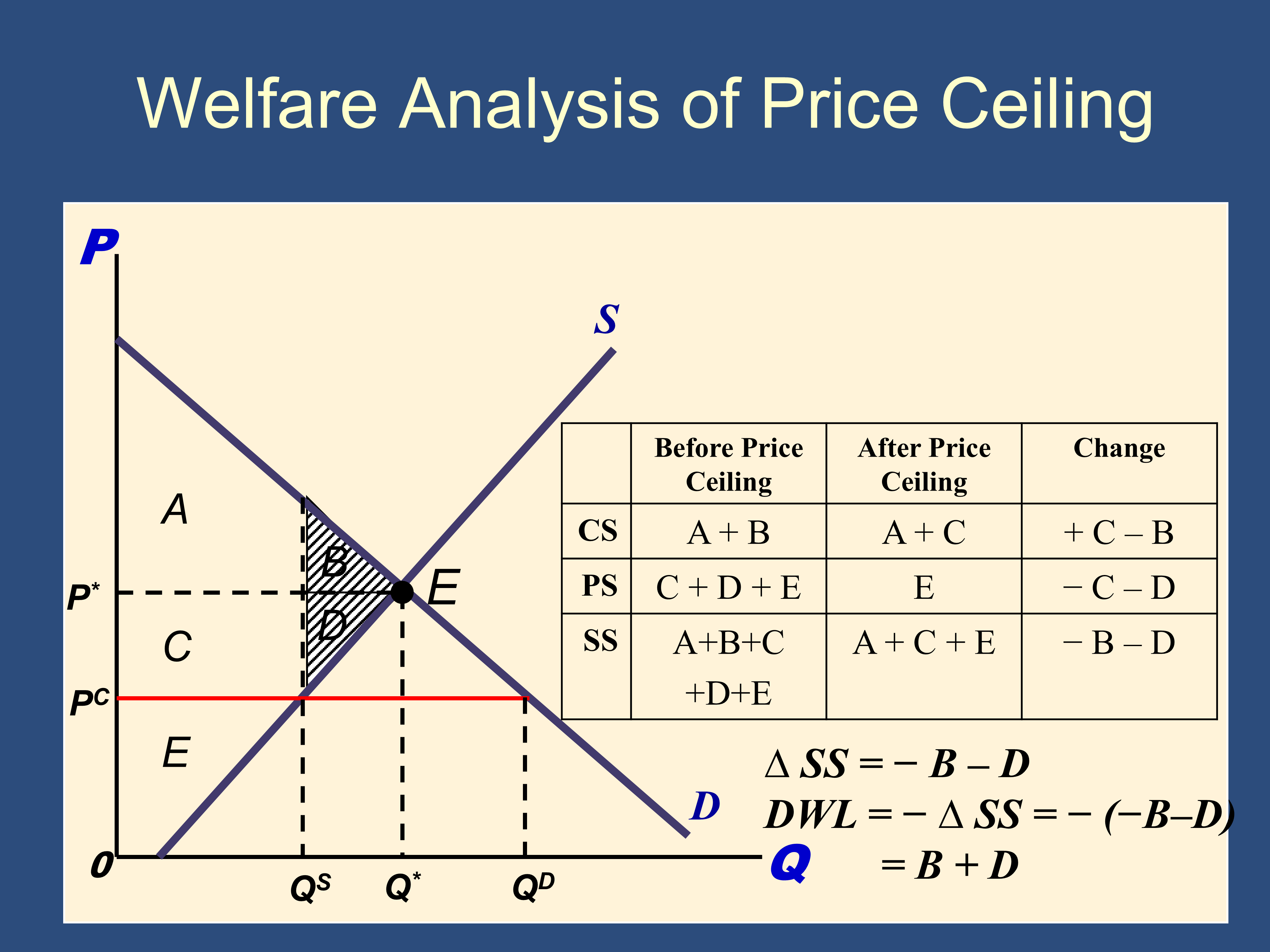
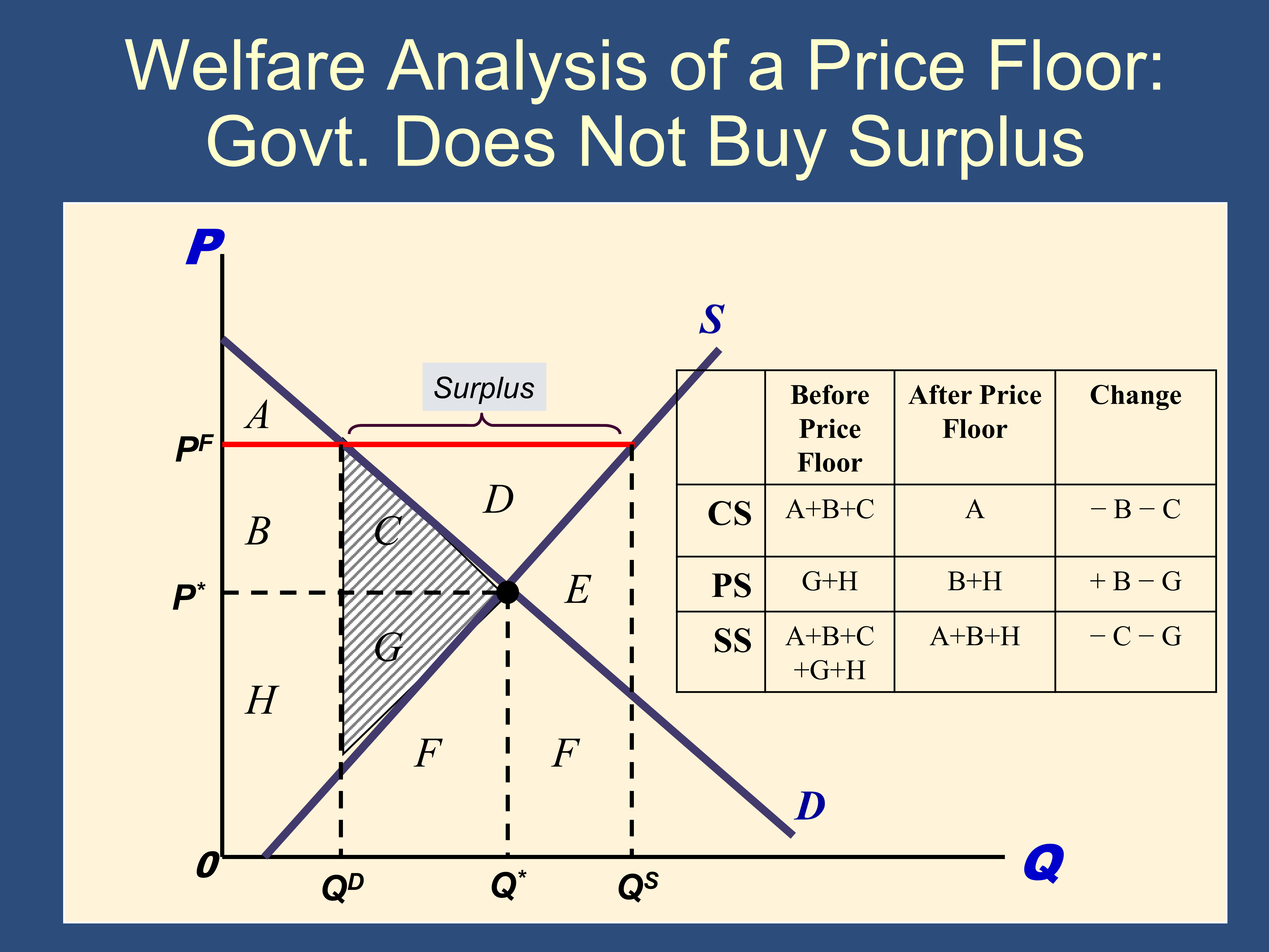
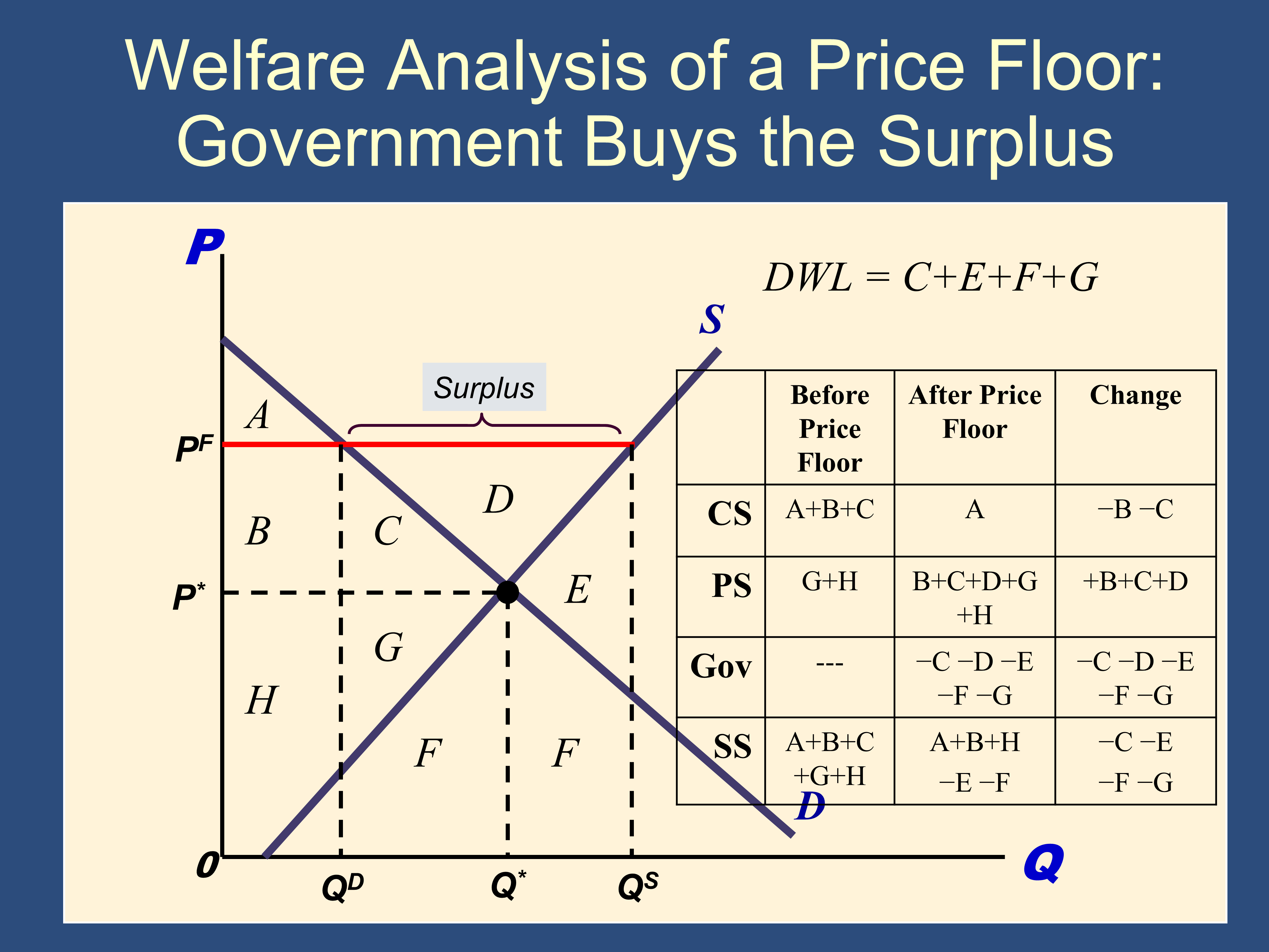
L9 – Welfare Economics

Consumer Surplus = Value to buyers - Price

• Value to Buyers = Marginal Benefit = Willingness to Pay = Demand Curve

Producer Surplus = Profit from selling the item = Amount received by sellers - MC

• MC = Willingness to Accept = Supply Curve

Total Surplus = Social Surplus = CS + PS
Economic Efficiency is the property of a resource allocation of maximizing the total surplus received by all members of society, i.e. social surplus.

Area of triangle = ½ (base × ht)

Pareto Efficiency (or Pareto Optimality) = A situation in which nobody can be made better off without making somebody else worse off.

First Fundamental Welfare Theorem = Any market equilibrium will be Pareto Efficient

References: 9 Apr 13.ppt and 9 - Notes

L10 – Externalities

In general:

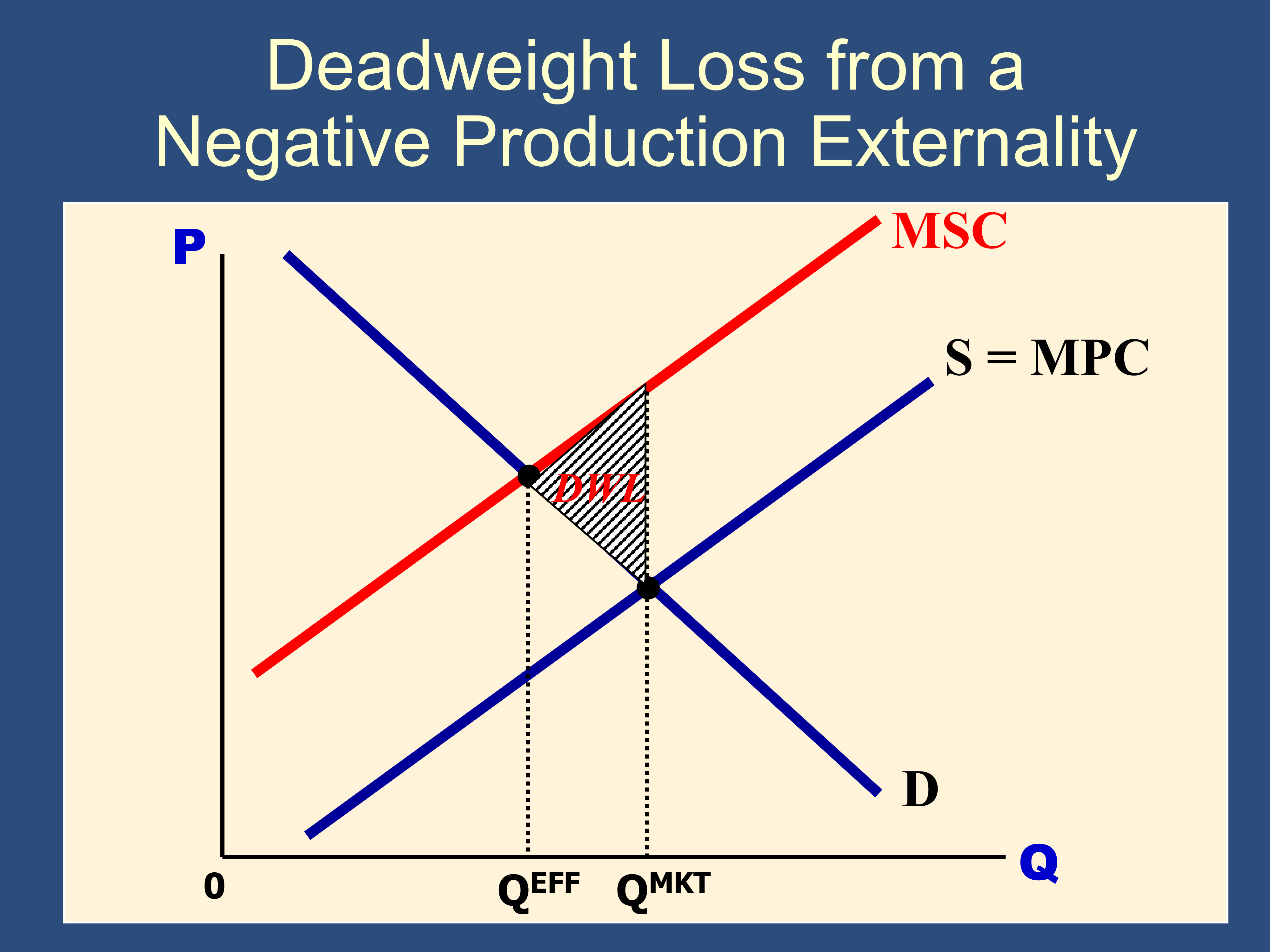
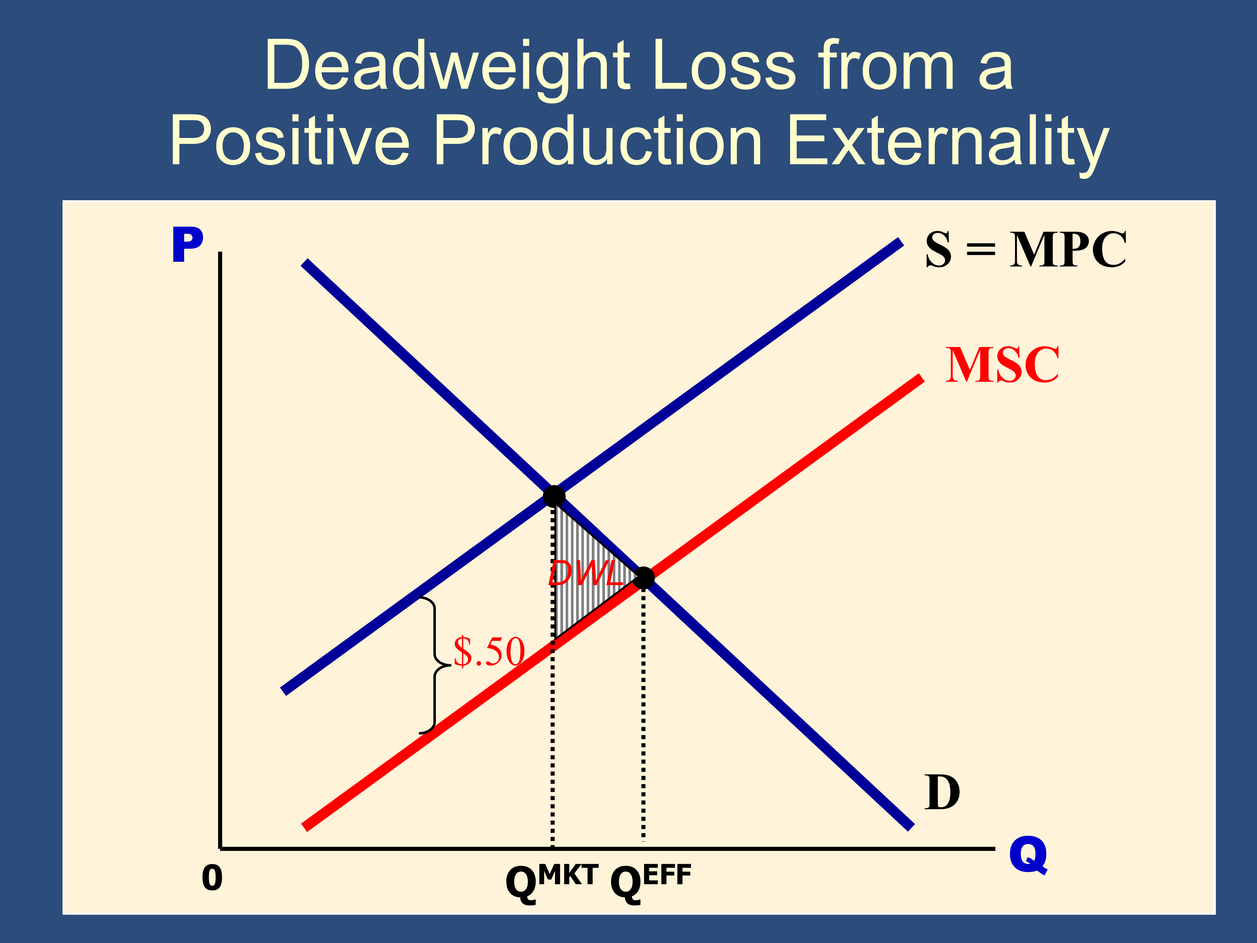
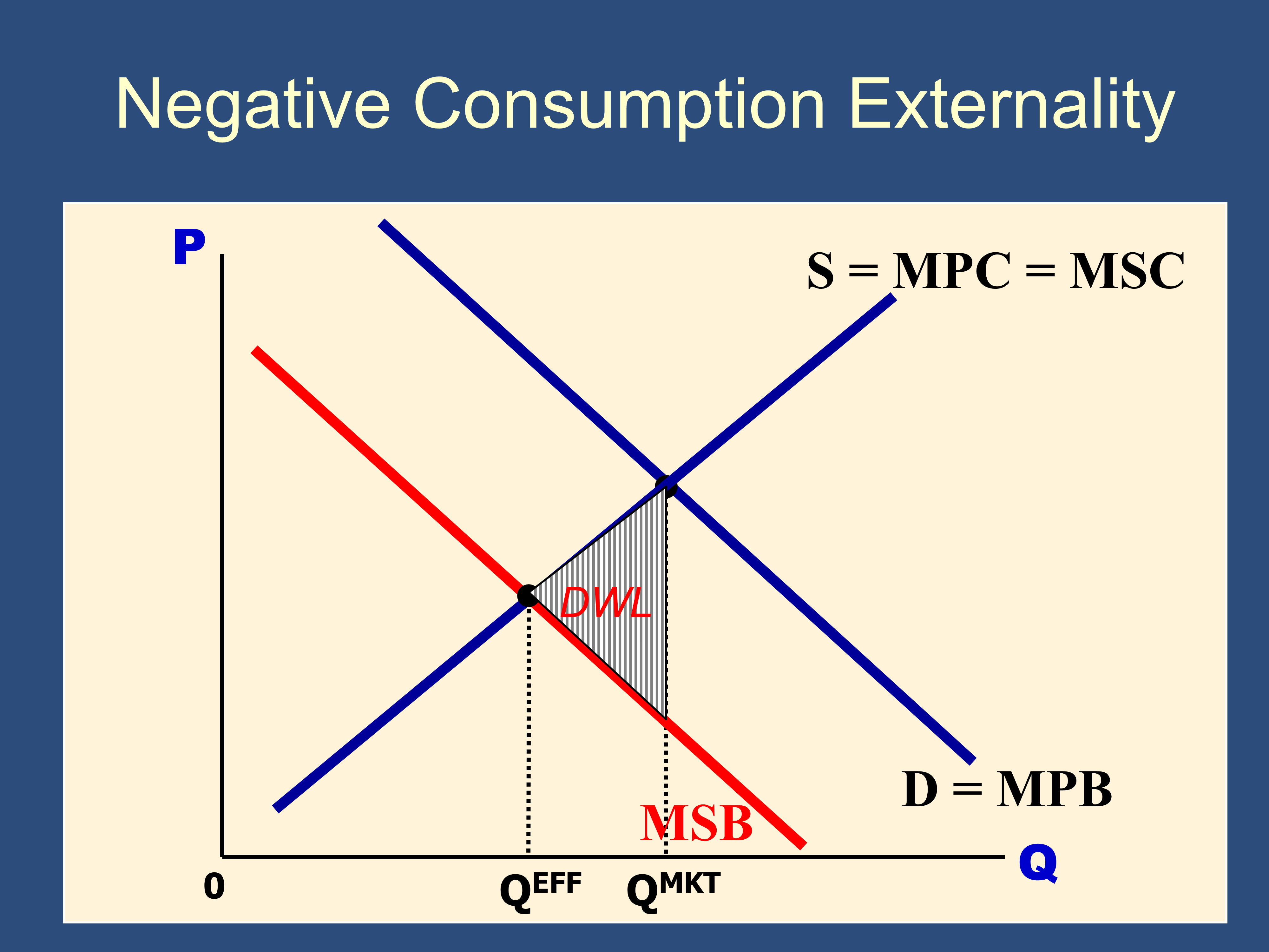
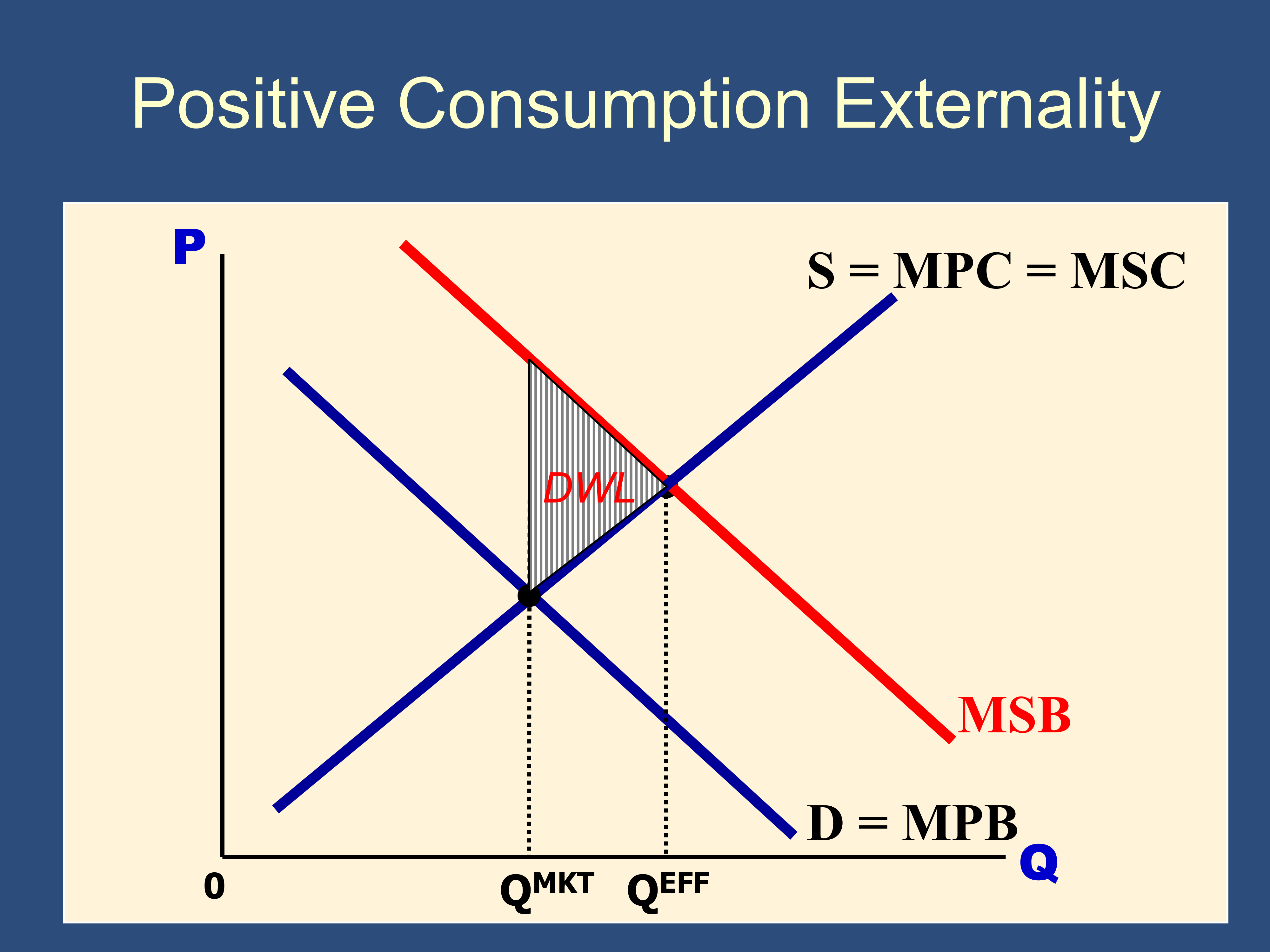
• Supply and Demand determine Q^MKT.
• The social optimum, Q^EFF , is determined by Marginal Social Benefit and Marginal Social Costs (MSB & MSC).
• Because people are self-interested, supply and demand are determined by Marginal Private Benefit and Marginal Private Costs (ie S=MPC and D=MPB).

	Production	Consumption
Negative	MSC > MPC MSC Curve Above MPC (or S) Curve QEFF < QMKT	MSB < MPB MSB Curve Below MPB (or D) Curve QEFF < QMKT
Positive	MSC < MPC MSC Curve Below MPC (or S) Curve QEFF > QMKT	MSB > MPB MSB Curve Above MPB (or D) Curve QEFF > QMKT

Negative Production Externality
Example: A polluting factory
Marginal Social Cost (MSC) = Marginal Private cost (MPC) + Additional Cost to Society

Positive Production Externality

Example: a university producing education has a byproduct of producing research. When you produce honey, you produce polinators for nearby plants.

Marginal Social Cost (MSC) = Marginal private cost (MPC) − Additional Benefit to Society

Negative Consumption Externalities

Example: Consumption of loud music. Second hand smoke. Alcohol.

Positive Consumption Externalities

Example: When you consume education, you become a better voter. When you consume yoga, you become kinder to the people around you.

Private Solutions to Externalities

• Moral codes and social sanctions
• Contracting between parties
  • Coase theorem: if transaction costs are low, private parties will bargain and achieve the efficient outcome.
  • Transaction costs are the costs that parties incur in the process of agreeing to and following through on a bargain

Government Solutions to Externalities:

• command-and-control policies.

• market-based policies.

  • Corrective/Pigouvian taxes are taxes enacted to correct the effects of a negative externality. Can “internalize” an externality.

  References: 10 Apr 20.ppt and 10 - Notes

L11 - Asymmetric Information

Violations of the Three Conditions for Perfect Competition:

1. Many buyers and sellers (Violations: Monopoly and Imperfect Competition)
2. Well-specified property rights (Violations: Externalities)
3. Complete information - well informed buyers and sellers (Violations: Asymmetric information)

I. Adverse Selection

• Definition: Any situation in which an uninformed party gets exactly the wrong people wanting to trade with her; there is an “adverse selection” of the (better informed) possible trading partners
• Occurs prior to a market transaction.
• Examples
  • Used car market (which gives rise to another term for adverse selection—the “lemons problem” - see below)
  • Market for insurance
  • Market for credit

Numerical example of Adverse Selection: The Lemons Problem

	Max price offered by buyers	Min price wanted by sellers	Probability
Peaches	$20,000	$17,000	50%
Lemons	$10,000	$8,000	50%

“The lemon dilemma”, The Economist, Oct. 11, 2001

Max buyer is willing to offer for any given car? They will be willing to pay the EV of their value of the car:
EV = 1/2 ($20,000) + 1/2 ($10,000) = $15,000
The maximum a buyer is willing to offer for any given car ($15,000) is less than the minimum ($17,000) that the seller of a peach wants for his car.
Result: Peaches will disappear from the market, and only lemons will be sold.
The market for Peaches will “unravel.”

1st Remedy for Adverse Selection: Screening

• Screening is the process by which an uninformed party attempts to gather information about the product or service offered by the informed party

2nd Remedy for Adverse Selection: Signaling

• Signaling is the process by which an informed party sends signals to uninformed parties conveying information about the quality of the product or service they’re trying to sell
• Signal must be effective in distinguishing between different levels of quality
• Signal will be more costly for a low-quality producer than for a high-quality producer
• Examples: Branding, Guarantees and warranties, Education, Signals on the job, Reputation, Gifts

II. Moral hazard

• Definition: the tendency of a transaction to change people’s incentives and therefore their behavior
• Occurs after a market transaction, and causes the people are doing business to be choose “bad behaviors.” For example, people may abuse rental cars or be less careful if they have insurance.
• Examples: Insurance market, on the job

II.A. Principal-agent is a subtype/variant of Moral Hazard

• Someone is supposed to be your agent, but their interests are different than yours and they do what is best for them. For example, employees shirk at work.
• Two conditions necessary for a principal-agent problem
  1. Asymmetric information—it must be difficult or costly for the principal to monitor the actions of the agent
  2. Divergent interests—principal and agent must have different interests or goals
• Some classic examples of Principal-Agent: employees shirking on the job, stock brokers guiding you to investments that make them wealthy rather than you, or a mechanic saying that you need repairs that you don’t need. These people should be acting in your interest, but act in their own interest instead.

References: 11 April 27.ppt and 11 - Notes