👨‍🏫 Notes on L7

Pindyck and Rubinfeld: pp. 369 – 377
 Section 11.2

See also: 🔎 Market Structure Comparison

Overview:

• Conditions for Monopoly
• Sources of Monopoly
• Demand and Marginal Revenue for a Monopoly
• Profit Maximization for a Monopoly
• Monopoly Power and Elasticity
• Price Discrimination
  • First Degree
  • Second Degree
  • Third Degree

Monopoly Definition: A monopoly is a firm that is the only seller of a good or service that does not have a close substitute.

How close?

• Electric utility
• Seafood restaurant

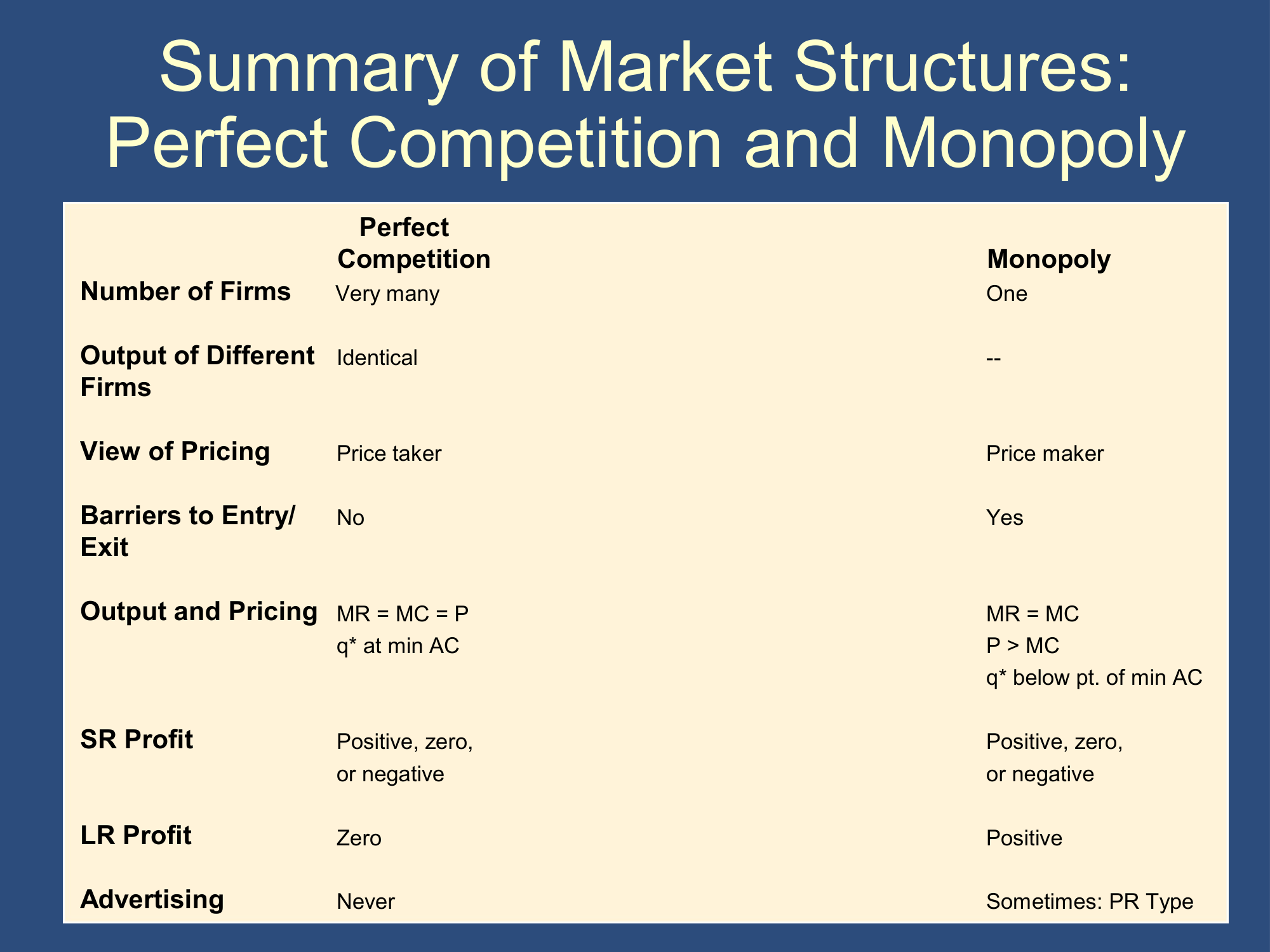
In contrast to perfect competition, in which there are many firms with identical products, in a monopoly there is a single firm offering the product. Examples include tap water and cable TV.

Conditions for Monopoly:

• One seller
• Barriers to entry

Sources of Monopoly

Bruce discussed four sources of monopoly:

1. Govt grant of a monopoly
2. Sole ownership or control of a scarce resource
3. Network externalities
4. Natural monopoly

Govt Grant of a Monopoly

• Public franchise
  • A government designation that a firm is the only legal provider of a good or service
• Patents and copyrights

Sole Ownership or Control of a Scarce Resource

• For many years, the Aluminum Company of America (Alcoa) either owned or had long-term contracts for almost all the world’s supply of bauxite, the mineral from which we obtain aluminum. Such control over a key resource served as a substantial barrier to entry for additional firms.
• The National Football League (NFL) acts as a monopoly in this manner too: it ensures that the majority of the world’s best football players are under contract to the NFL, and unable to be used for another potential league.
• De Beers
  • The most famous monopoly based on control of a raw material is the De Beers diamond monopoly.
  • De Beers sought to control as much
    of the supply of diamonds as possible, so it could keep prices high.
  • But by 2000, new competitors had eroded De Beers’ control of the world’s diamond production to 40 percent.
  • To maintain its monopoly power, De Beers introduced the “Forevermark” brand for its diamonds.

Network Externalities

• Economists refer to network externalities as a product characteristic whereby the usefulness of a product increases with the number of consumers who use it.
• Examples:        Auction sites (like eBay), Computer operating systems (like Windows), Social networking sites (like Facebook)
• These network externalities can set off a virtuous cycle for a firm, allowing the value of its product to continue to increase, along with the price it can charge.
• But consumers may be locked into an inferior product.

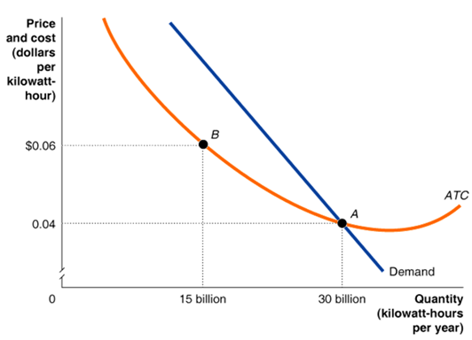
Natural Monopoly

• A natural monopoly occurs when economies of scale are so large that one firm can supply the entire market at a lower average total cost than can two or more firms.
• In the market for electricity delivery, a single firm (point A) can deliver electricity at a lower cost than can two firms (point B).
• Natural monopolies are most likely when fixed costs are high.

Marginal Revenue for a Monopoly

Profit maximization condition: For continuous quantities, produce that q for which $MR = MC$. So what is MR?

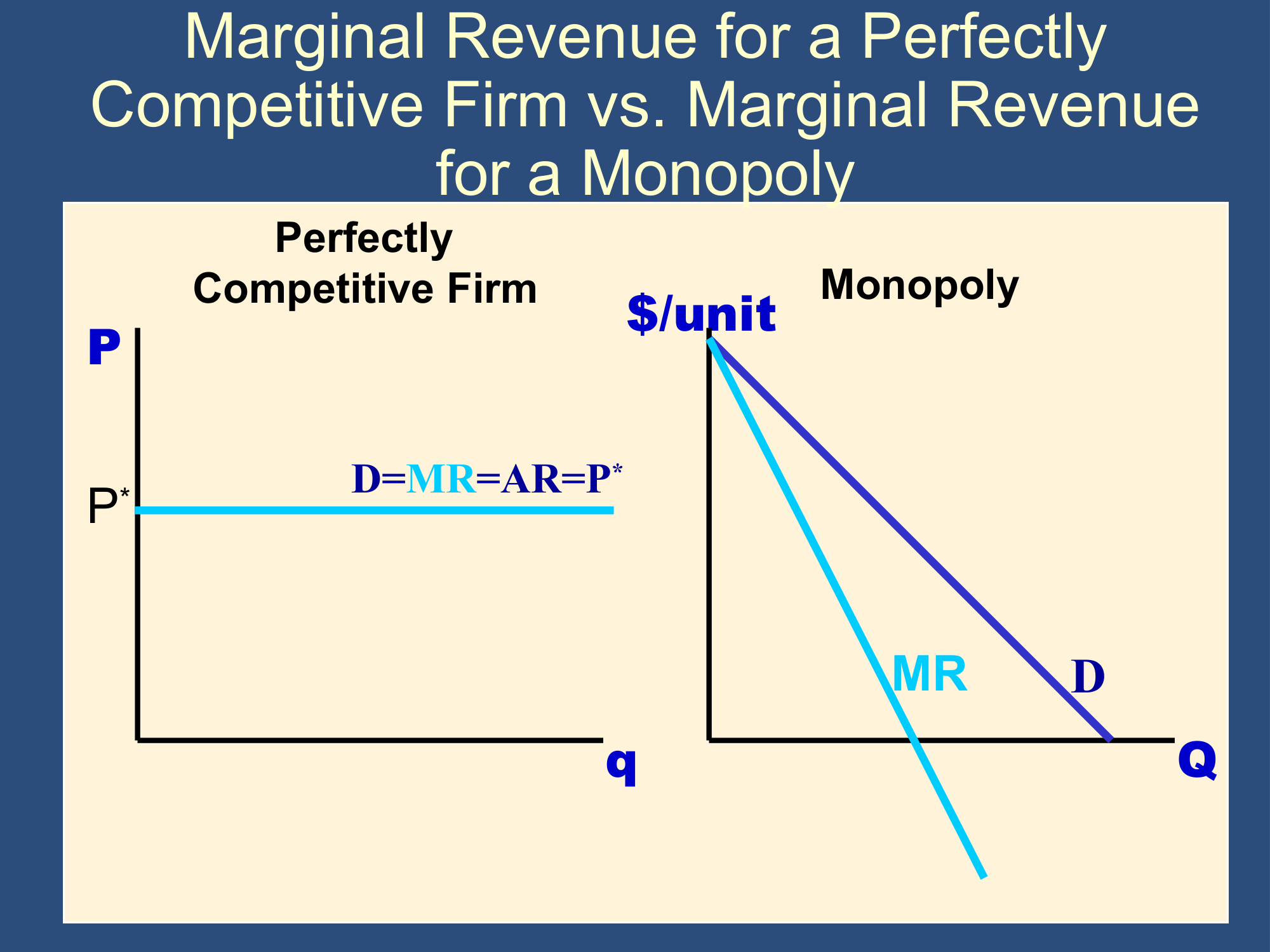
With perfect competition, $MR = P^* = D$, because competitive firms can sell as many units as they want for the market price, $P^*$
(they are a small part of market supply, so they won’t influence the market price)
With monopoly, $MR < P = D$, because to sell more units, a monopolist must lower the price on the units it is already selling
(they are 100% of market supply, so when they produce more, it lowers the market price)

Perfect Competition: $MR = P$
Monopoly and Monopolistic Competition: $MR < P$ ($= D = AR$)

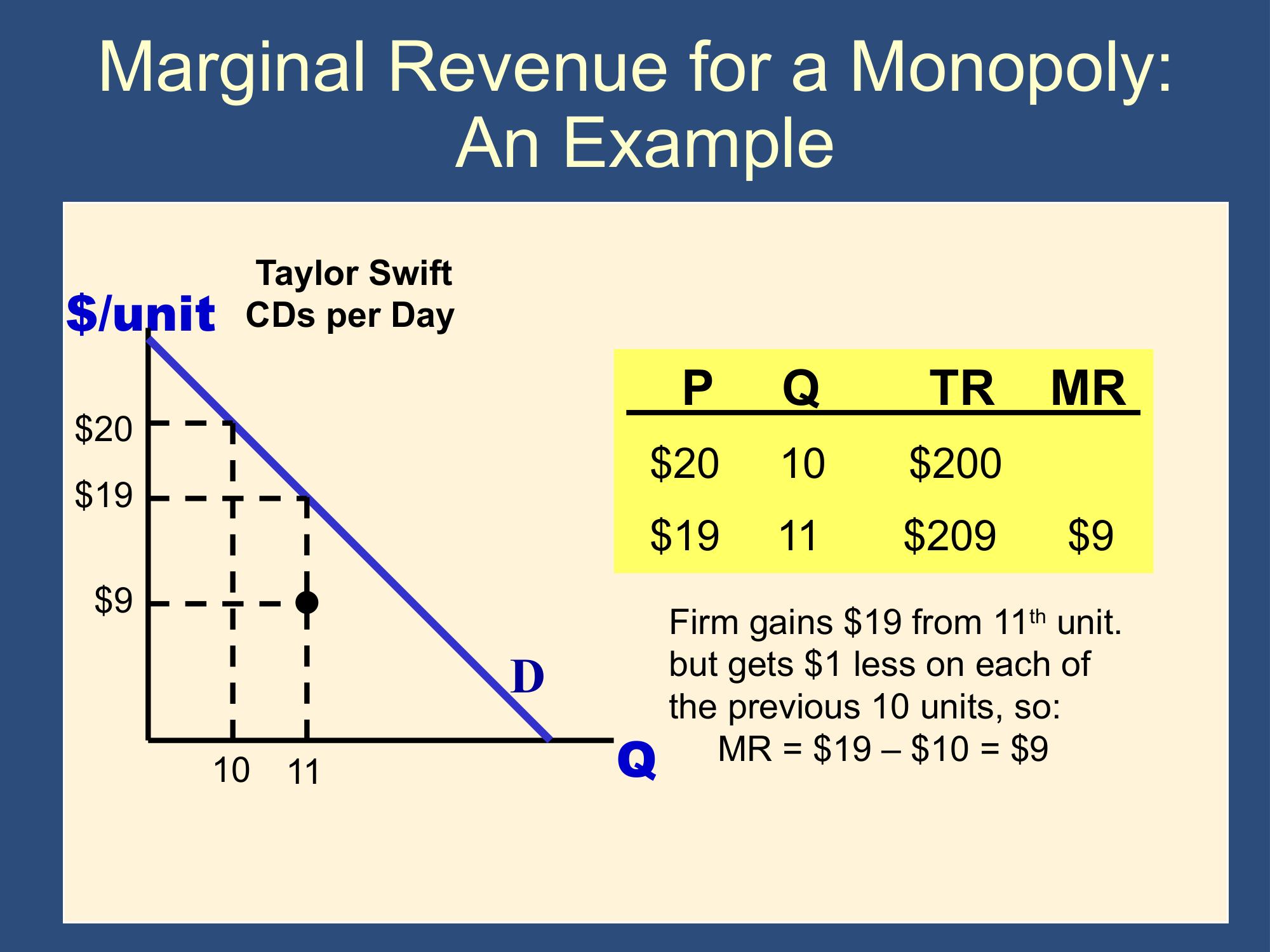
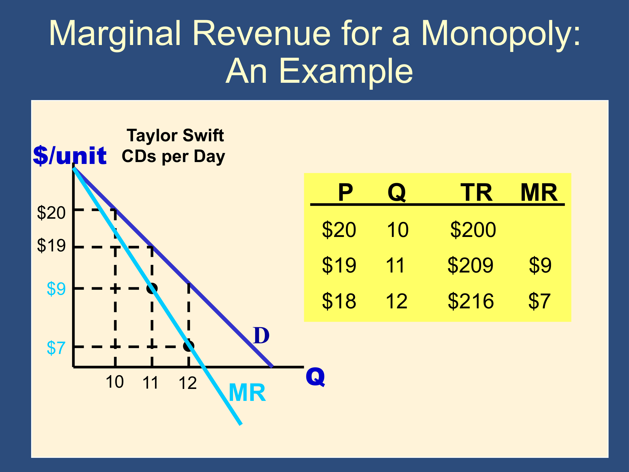
Example: (Note that $MR < P$)

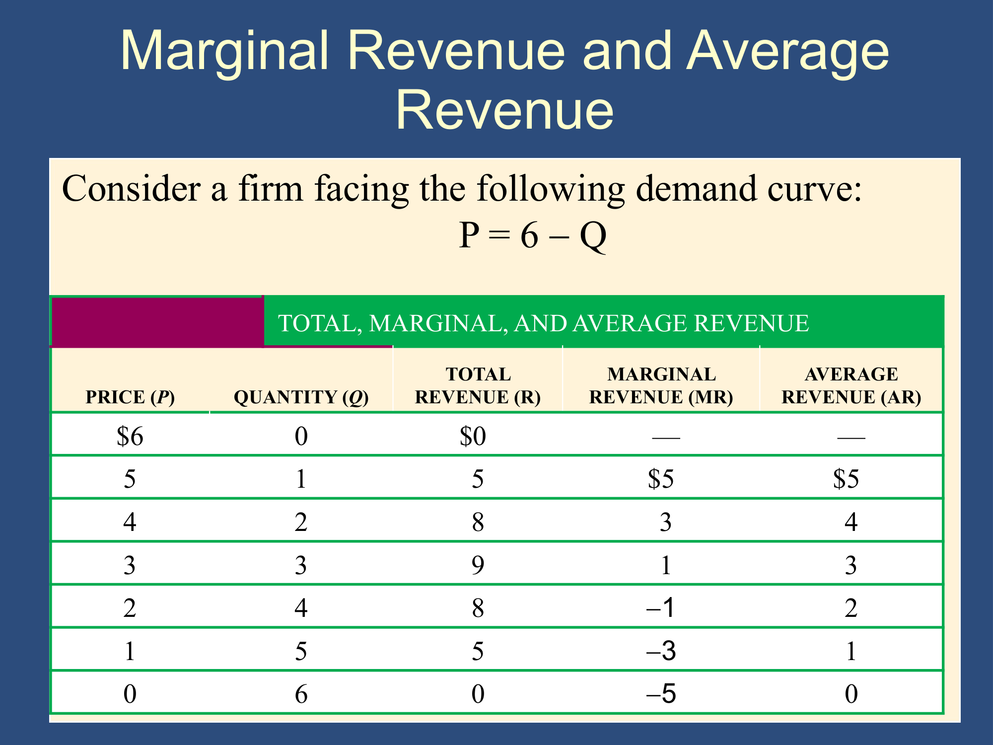
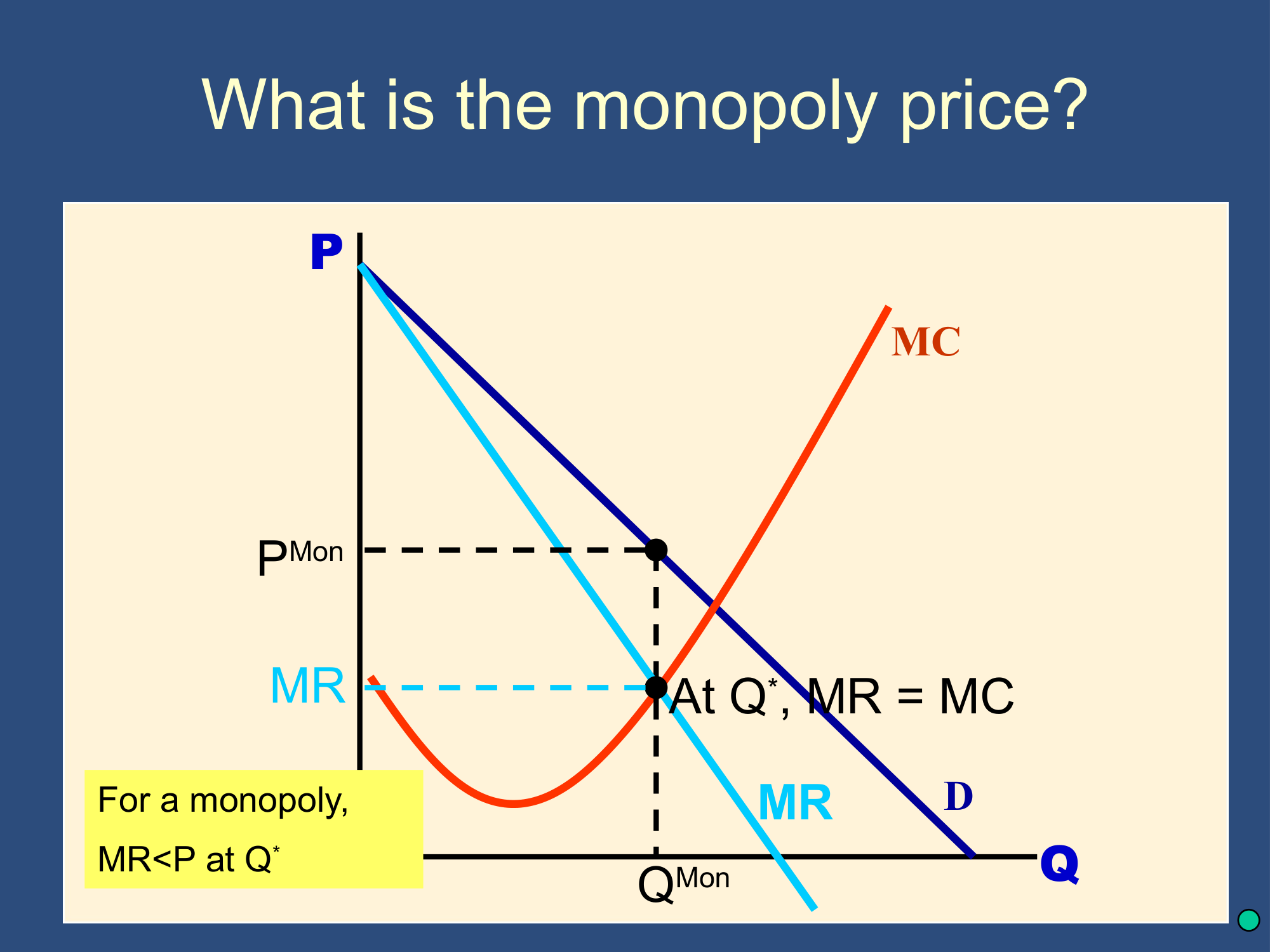
How to Solve a Monopoly Problem

1.) $MR = MC$ to figure out Q
2.) Draw a line up to the demand curve to figure out P
3.) Wrap up. $\text{Profit} = TR - TC = q^*(P - AC)$

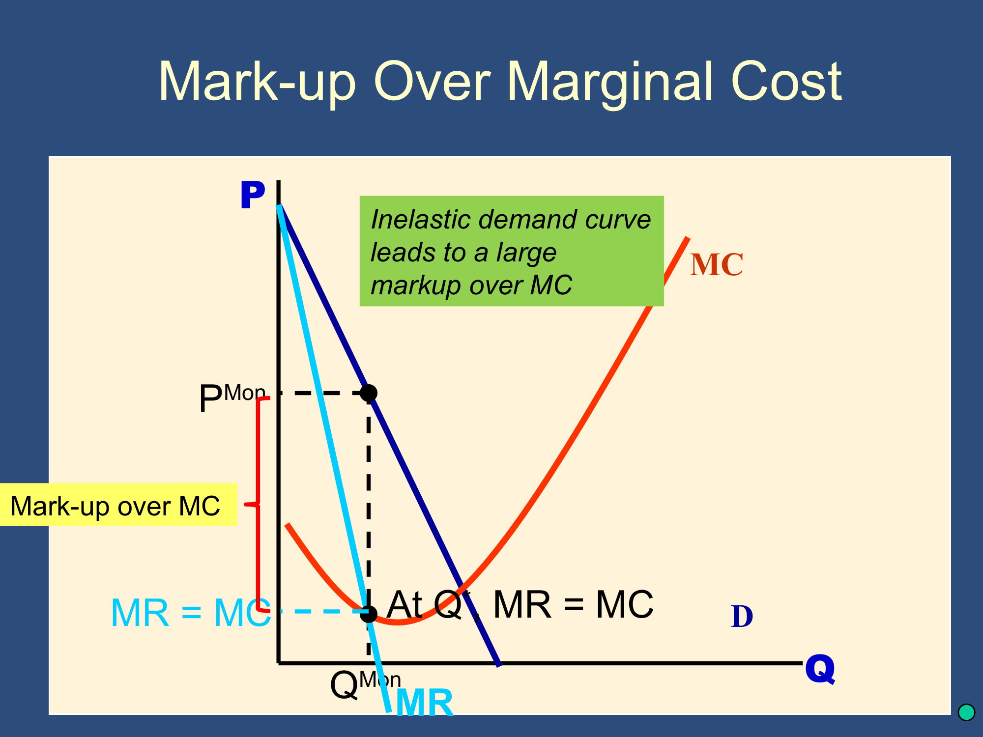
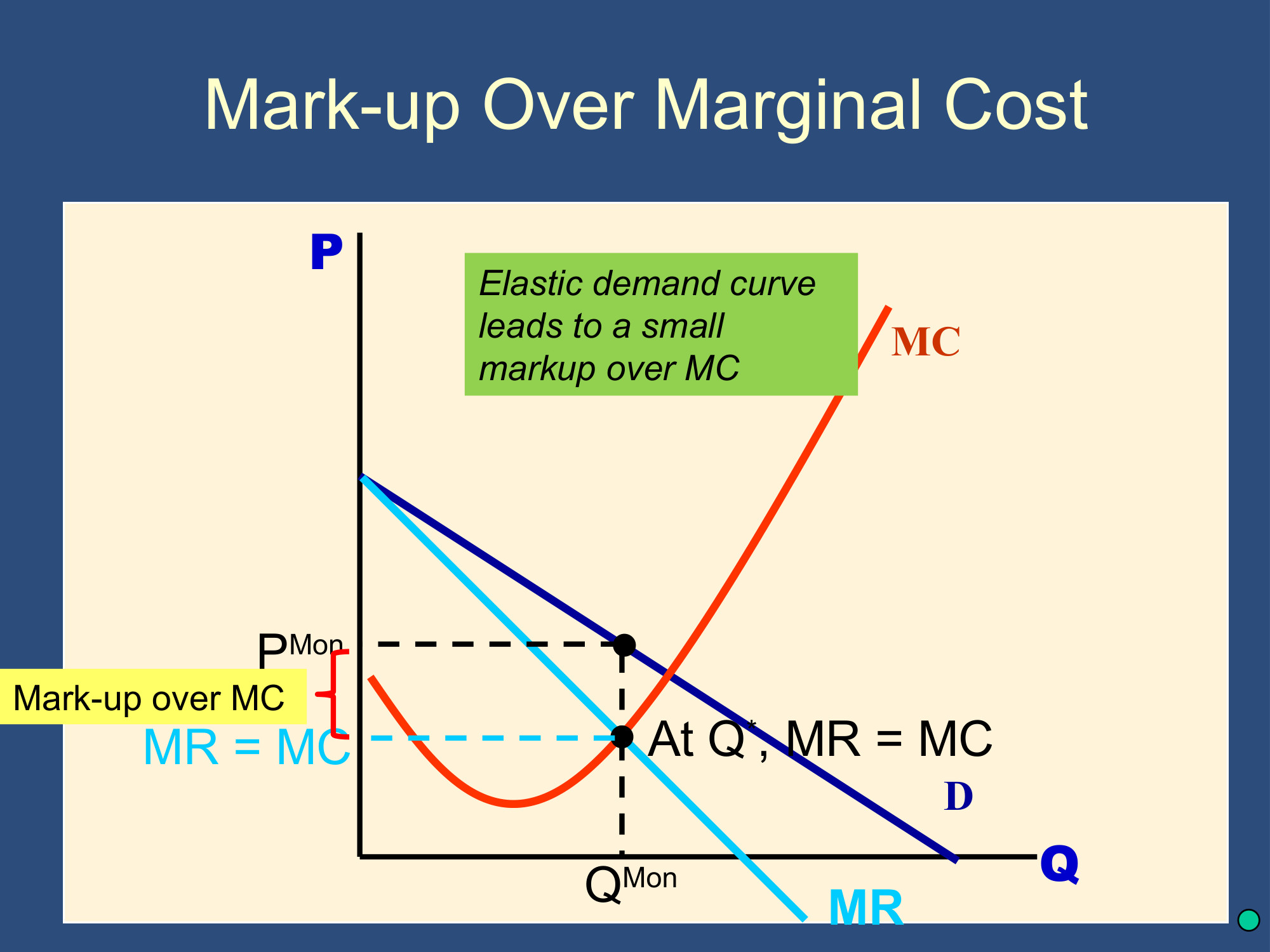
The Lerner Index measures what fraction of price constitutes the markup over marginal cost. $\text{Lerner Index} = \frac{P - MC}{P}$
If $P = 15$ and $MC = 5$, then $\frac{P - MC}{P} = \frac{15 - 5}{15} = \frac{2}{3}$. This means that 2/3 of the price is markup over marginal cost.
Elasticity, $E_d$, measures price sensitivity. When consumers are less price sensitive a monopolist has monopoly power and can mark up their prices above MC. This is illustrated by the following formula. It shows that the markup/Lerner index for a monopoly is determined by the price elasticity of demand:

$$\frac{P - MC}{P} = -\frac{1}{E_d}$$

The above formula can be derived using simple algebra that you’re not responsible for.

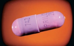
Astra-Merck Prices Prilosec example:

• In 1995, Prilosec, represented a new generation of medication for GERD (gastroesophageal reflux disease) and peptic ulcers. Prilosec was based on a very different biochemical mechanism and was much more effective than earlier drugs.
• By 1996, it had become the best-selling drug in the world and faced no major competitor.
• Astra-Merck was pricing Prilosec at about $3.50 per daily dose.
• The marginal cost of producing and packaging Prilosec is only about 30 to 40 cents per daily dose.
• The absolute value of the price elasticity of demand, $E_d$, is in the range of roughly 0.9 to 0.95.
• Setting the price at a markup exceeding 775 percent over marginal cost is consistent with our rule of thumb for pricing and elasticity.

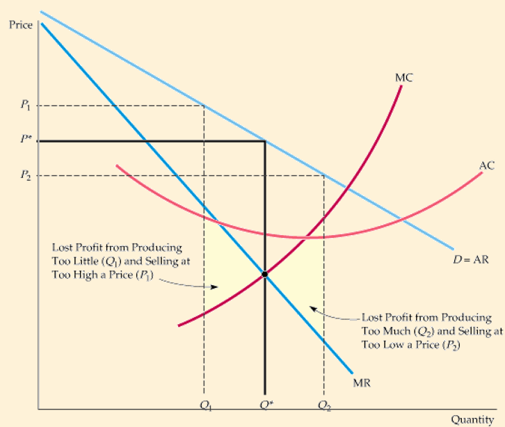
Understanding Profit Maximization for a Monopoly

PROFIT IS MAXIMIZED WHEN MARGINAL REVENUE EQUALS MARGINAL COST

• $Q^*$ is the output level at which $MR = MC$.
• If the firm produces a smaller output—say, $Q_1$—it sacrifices some profit because the extra revenue that could be earned from producing and selling the units between $Q_1$ and $Q^*$ exceeds the cost of producing them.
• Similarly, expanding output from $Q^*$ to $Q_2$ would reduce profit because the additional cost would exceed the additional revenue.

A Monopoly Has No Supply Curve

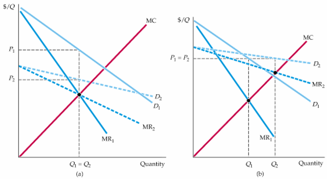
Shifts in demand

• Shifting the demand curve shows that a monopolistic market has no supply curve—i.e., there is no one-to-one relationship between price and quantity produced.
• In (a), the demand curve $D_1$ shifts to new demand curve $D_2$.
• But the new marginal revenue curve $MR_2$ intersects marginal cost at the same point as the old marginal revenue curve $MR_1$.
• The profit-maximizing output therefore remains the same, although price falls from $P_1$ to $P_2$.
• In (b), the new marginal revenue curve $MR_2$ intersects marginal cost at a higher output level $Q_2$.
• But because demand is now more elastic, price remains the same.

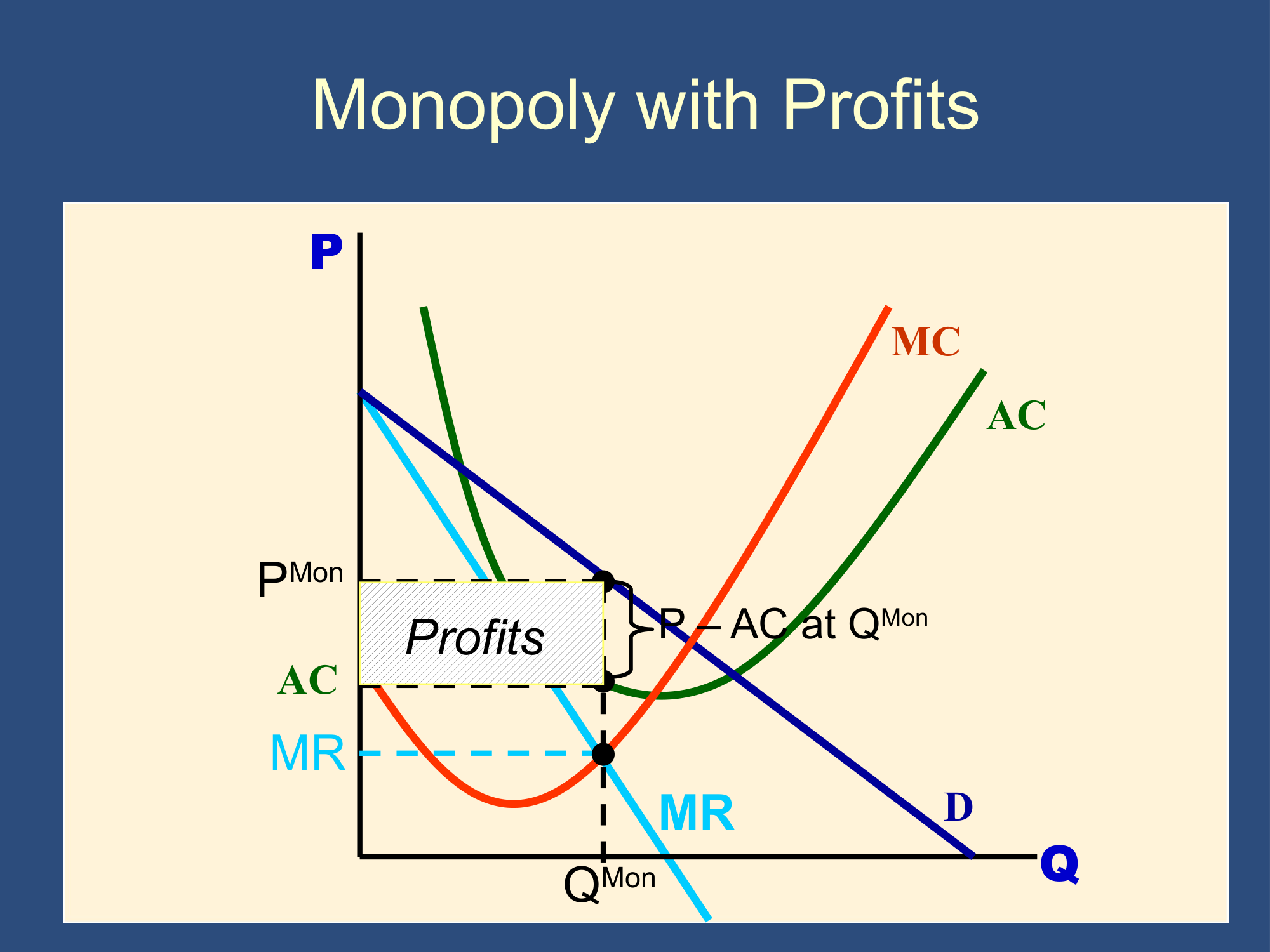
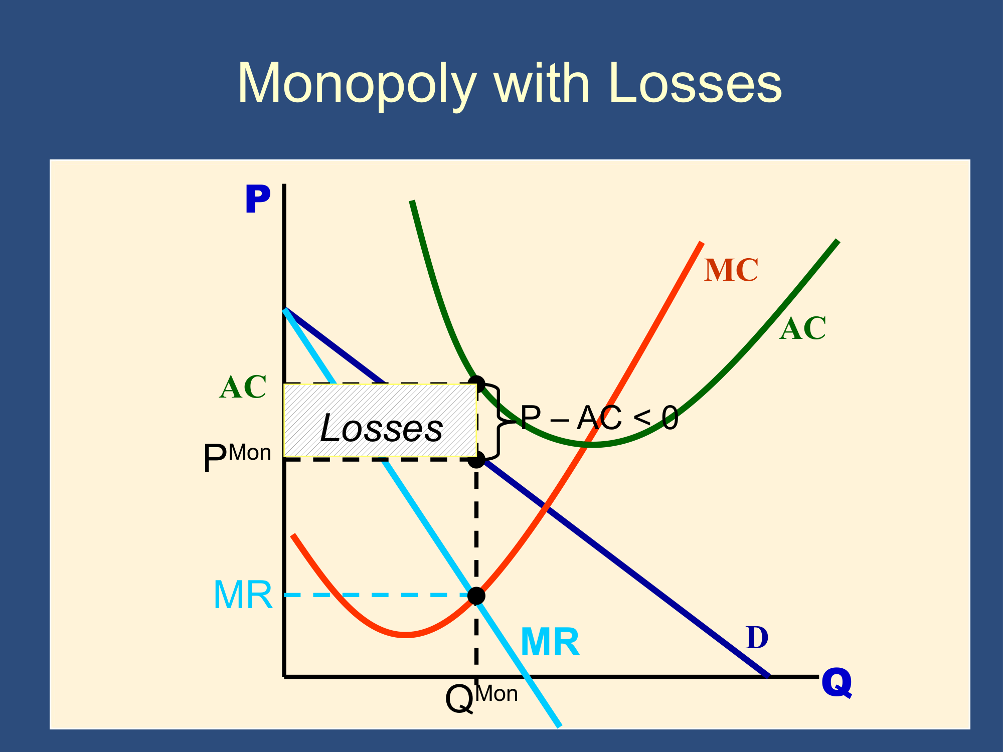
In the long and short run, monopolies can have profits, or break even.
In the long run, they won’t have losses because they would exit the market.

Price Discrimination

price discrimination- Practice of charging different prices to different consumers for similar goods.

• If a firm can charge only one price for all its customers, that price will be $P^*$ and the quantity produced will be $Q^*$.
• Ideally, the firm would like to charge a higher price to consumers willing to pay more than $P^*$.
• The firm would also like to sell to consumers willing to pay prices lower than $P^*$, but only if doing so does not entail lowering the price to other consumers.
• In that way, the firm could earn additional profits by selling to consumers represented by region B of the demand curve.

Three types of Price Discrimination:

1. First-degree (perfect) price discrimination: Practice of charging each customer her reservation price. (Reservation price is the maximum price that a customer is willing to pay for a good.)
2. Second-degree price discrimination: Practice of charging different prices per unit for different quantities of the same good or service. For example, block pricing is the practice of charging different prices for different quantities or “blocks” of a good.
3. Third-degree price discrimination: Practice of dividing consumers into two or more groups with separate demand curves and charging different prices to each group. For example senior & student discounts and coupons. This only works if the different groups have different elasticities so you can charge different prices to the different groups.

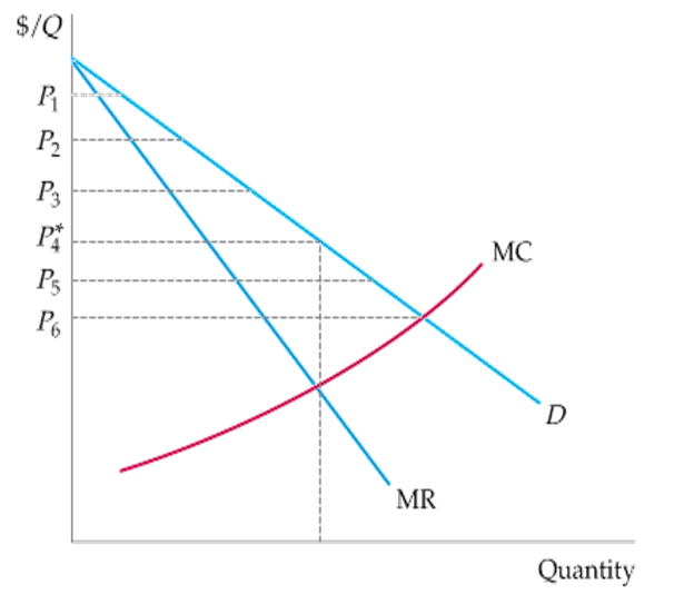
First Degree Price Discrimination

Practice of charging each customer her reservation price. (Reservation price is the maximum price that a customer is willing to pay for a good.)

The additional profit from producing and selling an incremental unit is now the difference between demand and marginal cost.

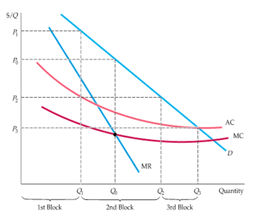
Second-Degree Price Discrimination

Different prices are charged for different quantities, or “blocks,” of the same good. Here, there are three blocks, with corresponding prices $P_1$, $P_2$, and $P_3$.
There are also economies of scale, and average and marginal costs are declining. Second-degree price discrimination can then make consumers better off by expanding output and lowering cost.

Third-Degree Price Discrimination: Creating Consumer Groups

- If third-degree price discrimination is feasible, how should the firm decide what price to charge each group of consumers?

1. We know that however much is produced, total output should be divided between the groups of customers so that marginal revenues for each group are equal.
2. We know that total output must be such that the marginal revenue for each group of consumers is equal to the marginal cost of production.

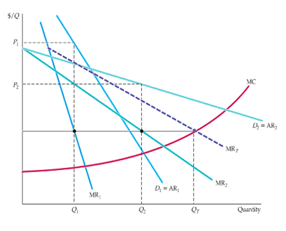
• Consumers are divided into two groups, with separate demand curves for each group. The optimal prices and quantities are such that the marginal revenue from each group is the same and equal to marginal cost.
• Here group 1, with demand curve $D_1$, is charged $P_1$,
• and group 2, with the more elastic demand curve $D_2$, is charged the lower price $P_2$.
• Marginal cost depends on the total quantity produced $Q_T$.
• Note that $Q_1$ and $Q_2$ are chosen so that $MR_1 = MR_2 = MC$.

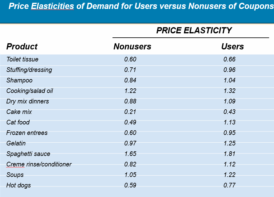
Price Discrimination and Coupons

• Coupons provide a means of price discrimination.
• Studies show that only about 20 to 30 percent of all consumers regularly bother to clip, save, and use coupons.
• Rebate programs work the same way.
  • Only those consumers with relatively price-sensitive demands bother to send in the materials and request rebates.
  • Again, the program is a means of price discrimination.

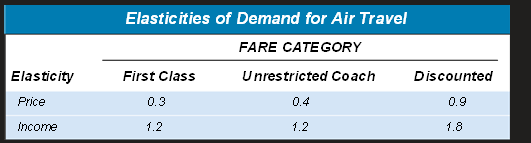
Price Discrimination and Air Fares

• Travelers are often amazed at the variety of fares available for round-trip flights from New York to Los Angeles.
• Recently, for example, the first-class fare was above $2000; the regular (unrestricted) economy fare was about $1700, and special discount fares (often requiring the purchase of a ticket two weeks in advance and/or a Saturday night stayover) could be bought for as little as $400.
• These fares provide a profitable form of price discrimination. The gains from discriminating are large because different types of customers, with very different elasticities of demand, purchase these different types of tickets.