🙋 Student Q&A (Lecture 4)

Click here to learn about timestamps and my process for answering questions. Section agendas can be found here. Email office hour questions to munger.e1010@gmail.com. PS1Q2=“Question 2 of Problem Set 1”

📅 Questions covered Thursday, Feb 26

🕣 10:18pm
❔ How to choose option 1 or 2? Is it based off the best amount? I thought there were more factors

✔ Individual consumers will always choose the option that has the highest expected utility. Firms may choose the option which gives them the highest expected value of their profit. Though he doesn’t tend to ask questions like that, mostly all the questions which get asked are about maximizing the highest expected utility for an individual consumer.

🕣 10:19pm
❔ go over risk adverse graph and all the variables

✔in video

🕣 10:19pm
❔ when it comes to insurance the first example of medical insurance i am not too sure where bruce got the $10,000 from and why is it $30,000? Shouldn’t it be 90% of $30,000?

✔earlier in video

🕣 10:20pm
❔ want to be careful when drawing EV and then CE and when the line should stop? (slide 39)

✔Follow the 4 step process! see video

🕣 10:22pm
❔ When you have EV how do you calculate EU? Do you look at the graph and see which line over hits the utility curve?

✔ See 4 step process

🕣 10:22pm
❔ The wording of insurance questions how to read these properly or is it just practice? What is the information given about being disabled or sick and then what is the cost..? What does the person will earn 0 dollars does that mean the insurance covers everything?

✔just answered.

🕣 10:25pm
❔ willingness to pay=H-CE? Can you explain H?

✔H is the best outcome.

🕣 10:25pm
❔ can you go over how to get CE in a problem and on a graph? Still confused…?

✔ 4 step process.

🕣 10:26pm
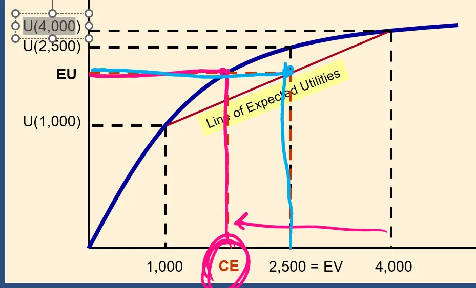
❔ Can you walk through steps how to get util of the insurance policy and then the consumers’s EU with no policy? These are hard steps and how to pick what goes with what?

✔ For the util with the insurance policy use the “blue line”. For util without, use the straight “red line.”

🕣 10:28pm
❔ trouble IDing what the question is asking EV, EU, CE etc… ?

✔

🕣 10:28pm
❔ I am still trying to grasp the EV/EU/CE correlations and how they are applied the different risk types. Can we go over those slides again tonight?

✔ covered earlier.

🕣 10:32pm
❔ Can we also talk about insurance and the example problem from lecture with Ben and home insurance?

✔ covered briefly; can return to.

📅 Questions covered Sunday, Mar 1

🕣 7:47pm
❔ Interpretation: Q9, how good does the curve have to be?

✔ Not very.

🕣 7:53pm
❔ What’s coming up on the exam?

✔ The following page is not ready to be published, but you can see my current working draft here.

🕣 8:14pm
❔ When is the paper due?

✔ Mar 2nd 11:59pm

🕣 8:15pm
❔ I would also like to have some practice problems recognizing the different risk types when given certain or limited key pieces of information. For example: Ben does X, Y, Z or Ben decides to accept this offer/option. What risk type is he most likely?

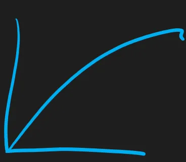
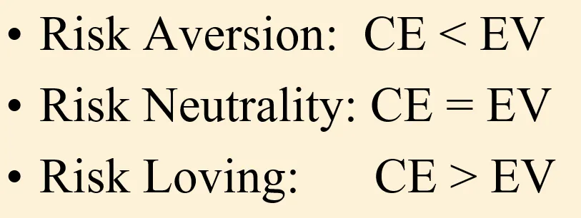
✔ Most people are risk averse. Therefore, most utility functions curve downward.

If a question requires you to assume that they’re risk averse, I think Bruce is going to say they’re risk averse. That’s all we know. You can only reason from what’s true, and that’s all that’s true. He knows what you know, and he knows what you don’t know, and all questions are going to be fair and solvable.

If Rob always rejects a fair bet, then we know that he is risk averse.
If Rob always accepts a fair bet, then we know that he is risk loving.
A bet is considered fair if your expected value from playing the bet is zero.
If someone always accepts a bet when it has a positive expected value and always rejects a bet when it has a negative expected value, that person is risk neutral.

Suppose we play a game. If a fair coin comes up heads, then I give you a dollar. If it comes up tails, then you give me a dollar. What’s the expected value to you for playing this game?

There is a 50% chance that you will win a dollar, and a 50% chance that you will lose a dollar.

EV = 50%*$1 + 50%*(-$1) = $0 on the other hand, let’s suppose that the coin wasn’t fair and that there was a 51% chance that it will come up heads. EV = 51%*$1 + 49%*(-$1) = $0.02 (I think)

high-frequency trading and a lot of the actual trades that are made on stock markets right now basically amount to this. You have computers making millions of trades like this, since each one has a positive expected value of two cents. If you make a million trades, then you’ve made $20,000, and if you just keep on doing that in many places, if you do scale it up to billions, then you’re minting. You’ve got a mint.

🕣 8:23pm
❔ Can it also be- If robs utility reduces when his income rises = risk averse

✔ It can’t. We’re going to generally assume that everyone’s utility increases when their income rises. In economics, we try to start with assumptions which we feel are reasonable, and in general it’s pretty common for us to assume that more. We are always going to assume that the marginal utility of money is positive. Risk aversion and risk loving behavior are slightly different from this.

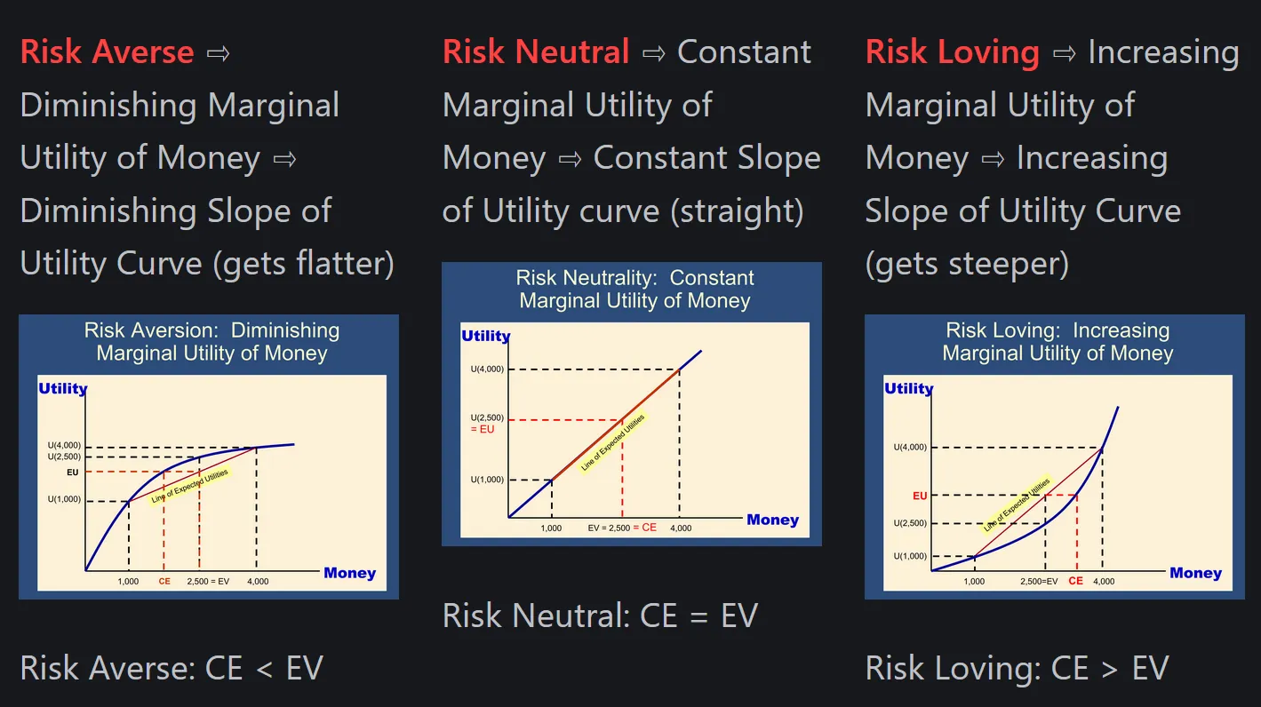
Above, we see that
Risk Averse = diminishing MU of money
Risk Neutral = constant MU of money
Risk Loving = increasing MU of money\

Above, we asserted that, because everybody likes money, your utility always increases whenever you get more money. That means that the additional utility you get from an additional dollar is always positive. I’ve just quoted the definition of marginal utility. It’s shown that the marginal utility of money must always be positive. Therefore MU>0

🕣 8:30pm
❔ In this practice question, in order to find if $5.2 certainty is better or if option B is better. You calculated EU as × EU (B) = 80%×12 + 20%×23=14.2 but just before that we calculated EU (B) as EU(Ticket B) = 75%×U($2) + 25$10) = 75%×12 + 25%×24 = 15 utils.

Why did the probabilities change? And how are we getting EU of $5.2 is 18.2 utils? (its not mentioned anywhere).

The way I was approaching this question is I found out the EV of B which we know is $4. Then I saw the graph and $4 has a EU of 15 utils. And then plotted $5.2 on the graph which would be more than 15 utils. And since $5.2 will give more utils we chose $5.2. Why is this approach incorrect?

✔ The original OneNote version of this website started off just as materials that I made during class. That’s why, on the homepage of all my websites, I’m always very clear: this just started with stuff that we would draw and problems that we would make up during section. There’s going to be little residues of that. I think this is one of the residues of that. I think it’s going to take a lot of work to see if I can find where was the problem that that came from. That’s what we’ve got for right now.

🕣
❔ a. In the first question, part D it says: Premium = best − C E = $ 100 − $ 30 = $ 70 Premium=best−CE=$100−$30=$70. I’m not sure where you got 100 and 30 from?

✔Skip these exercises.

🕣
❔ b. The second part of the question says without insurance her EU is 51 utils. How did we calculate this since it doesn’t show on the graph.

✔Skip these exercises.

🕣
❔ If a candidate get a fixed job offer for $100000. The expected utility for $100000 is fixed at UE(100000). This is clear. If a 2nd job offer has a fixed salary amount of say $50000 and a potential profit sharing bonus of $100000 but a 50% chance of getting it, how do you calculate the UE? Is it $50000 + (100000)(0.50) = $1000000 EV and then cross over to the UE? or is it we do the UE(50000) + (UE50000)×.75? This is where I get super confused.

✔

Could we calculate CE without having the util values?

✏️ Suppose that I get
5 utils from $5,
6.5 utils from $6,
7 utils from $7,
7.6 utils from $8,
8 utils from $9

Suppose that I have a ticket that has a 1/3 chance of paying $5 and a 2/3 chance of paying $9. What is the certainty equivalent? ✔CE is the amount of money that a person is willing to take instead of taking the gamble. You are indifferent between the CE and the gamble. Indifferent just means “same utility.”

Therefore, our definition of the certainty equivalent is that the certainty equivalent is a specific, certain amount of income such that u(CE) = EU(gamble) EU(gamble) = Prob×util + Prob×util = 1/3×u($5) + 2/3×u($9) = 1/3×5utils + 2/3×8utils = 5/3+16/3 = 21/3=7utils Coincidentally, $7 also gives them 7 utils. Therefore, u($7) = EU(gamble) = 7utils

Therefore the CE is $7.

Let’s see if we can guess whether the EV is higher or lower than this CE?

Ah, we need to know if they are risk averse/neutral/loving.

We can calculate MU
5 utils from $5,
6.2 utils from $6, MU of sixth dollar = 1.5utils= Δutil/ΔQ = (6.2utils-5utils)/($6-$5) = 1.2utils/$
7 utils from $7, MU of seventh dollar = (7-6.2)/(7-6)=1.2
7.6 utils from $8, MU = (7.6u-7u)/(8-7)=.6u
8 utils from $9 = .4u Risk Averse because diminishing MU.

✏️ Suppose that Joe gets
5 utils from $5,
6.5 utils from $6,
7 utils from $7,
7.6 utils from $8,
8 utils from $9

Joe is
A. Risk Averse
B. Risk Loving
C. Risk Convex
D. Risk Neutral
✔ First, ID option C as a red herring.

🕣 9:16pm
❔ Would it be best to review PSETs and manipulate the problems like change the numbers? Or asks if price rise make the question if the price drops? Etc…. I know there are problems in pearson but those might have information we are not going over….

✔ I think that adjusting the problem set questions to create new practice questions is a great idea. It requires a strong grasp of the material, so I would not attempt it until you are advanced in your studying. The first steps are what I’ve described at the start of this section.

1. Make sure you really understand the concepts in the slides.
   • One way that I used to tell people to study the slides is to, for each slide, see if you could explain it to your grandparents. Could you explain each slide in such simple language that it would make sense? We illustrated how very important that is today when we covered certainty equivalent. Many of you had a definition of certainty equivalent and you could use it for certain problems, but you didn’t necessarily know the core intuition of certainty equivalent, which is the amount of money where you’re indifferent between the gamble and getting that money. That’s fundamentally what it was. The “explain it to your grandparent” exercise would have paid off in that particular, very stressful problem.
   • Use the slides as flash cards
2. Redo all problem sets. Do questions in my website. Once you’ve done those things, then I think you can start working on what you’re describing and making your own problems. I think it would be very productive. We could also try that just for fun. I could set up a live stream (what I call live streams), where we just kind of hang out and do problems. You can also just say, “Hey Rob, can we do a live stream?” I’d be happy to make problems; can we just hang out and make up problems, you make up problems and we work on them together? I’m happy to do those also.

🕣 9:24pm
❔ Suppose your net worth is $200K and I offer you a bet. You can provide a fair coin (I’ll test it to ensure fairness). We’ll flip it fairly. If you win the coin toss, I give you $220K. If you lose the coin toss, you give me $200K.

The EV of this gamble is 50%×$220,000 + 50%×(-$200,000) = $10,000

But a typical person is risk averse and wouldn’t accept the bet.

Background: If a bet has an EV of 0, it is a “fair bet” If a bet has an EV > 0, it is a “winning bet” If a bet has an EV < 0, it is a “losing bet.”

If an expected utility maximizer is offered a winning bet, like the one above, and they reject it, it is because they are risk averse in the relevant portion of their utility function.

If someone is offered a losing bet, and they accept it, they are probably risk loving (in the relevant portion of their utility function).

Can you explain this part? Max EU I am having a hard time locating?

✔ Unlike most things in this course where you should know why something is true, these particular facts above are just facts that I’m telling you. Many times Bruce will show you the proofs for things that he tells you, and that gives people a sense of confidence. That’s why he does the proofs. You feel like you get it.

For these particular facts, I’m just asserting, and I’m not going to burden you with the proofs, so you can just trust me on it and not worry about it. Just kind of understand what it means. If I’m trying to figure out if someone is risk averse, risk loving, or risk neutral, if I’m given a couple of bets, I can calculate whether they’re fair, winning, or losing bets, and I can figure out whether they’re risk averse on the relevant portions of the utility curves.

The reason we’re not giving you the proofs is that I suspect that they involve fancy math having to do with how curves are curved. If you have a concave curve, then certain things happen when you’re taking expected values. We just don’t want to burden you with that.

We want to be able to talk about how uncertainty and risk-taking is handled in economic context and how economists think about that. We don’t want to make a prerequisite of this course have advanced math. Here, I guess we’re stuck with just asserting it, and that’s all we can give you.

🕣
❔ 1. On slide 56, it says that based on Scottie’s choice, we calculated his EV at $13.5M and then concluded that his CE must be more than $15M but less than $17M. I’m unable to understand how we came to that conclusion based on the EV and the choice made by Scottie?

✔ If we know that Scottie is risk averse, then his CE must be more than 13.5M

The definition of CE is that u(CE) = u(Gamble). EV of gamble is 13.5 He could have gotten 15 for sure. Because he chose the gamble, it must be that EU(Gamble)>EU(the other option), ie that EU(15m)<EU(Gamble)=EU(CE) Therefore, the EU(15m)<EU(CE) Because more money is better, if EU(15)< EU(CE), then the CE must be greater than 15 million.

Also, the CE is always lower than the best outcome because more money is always better.

🕣
❔ 2. I was going through some practice exams on Myeconlab and came across the below question. Can you help me understand this please? I’m not sure why he would be on a higher IC. Also, this problem is very time consuming, can we expect something like this in the exam?

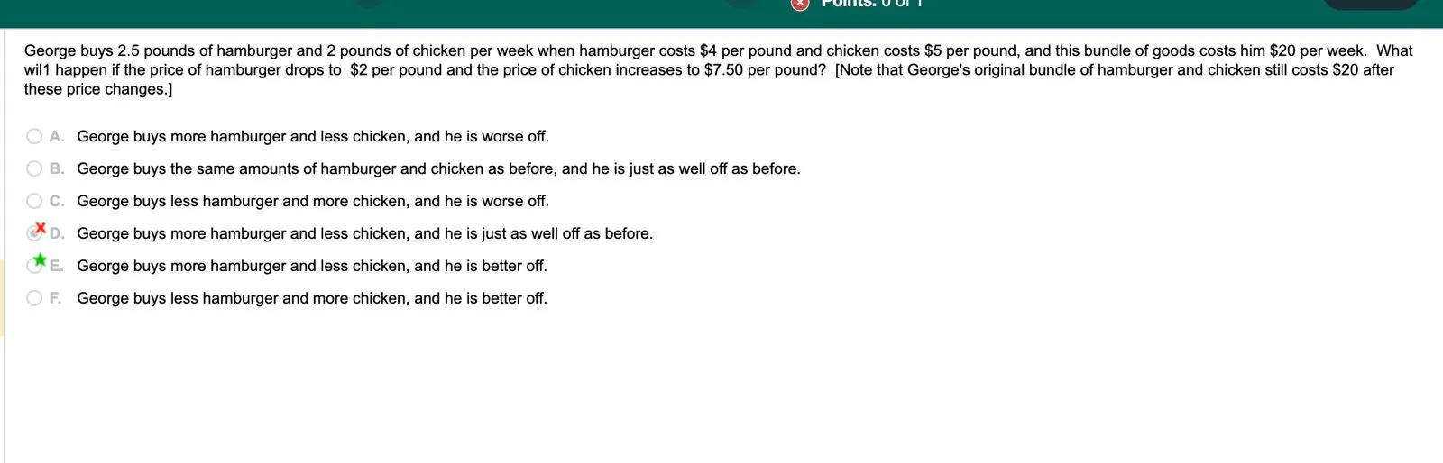
✔ don’t worry about this. The way that this is set up is designed to isolate the substitution effect. Because chicken became relatively more expensive, he’ll buy less chicken (and correspondingly more hamburger).

Because he could still afford the old basket of goods that he was purchasing previously, it must mean that the new basket of goods makes him better off than the old basket of goods, or else he wouldn’t have switched. Therefore we can reasonably conclude that the new basket of goods makes him happier than the old basket of goods, or at least as happy as he was before and probably more happy because he bothered to switch. More precisely: u(old basket)≤u(new basket)