👨‍🏫 Notes on Lecture 10

Lecture Outline

• Introduction to Externalities
• Production Externalities
  • Negative
  • Positive
• Consumption Externalities
  • Negative
  • Positive
• Private Responses to Externalities
  • Coase Theorem
• Public Responses to Externalities
  • “Command and Control” Responses
  • Pigovian Taxes

Concept Introduction

Fundamentally, externalities are about people being selfish. There are spillover effects on other people (aka external effects or “externalities”). However, decision makers don’t take those effects into account when they decide how much to produce or consume.

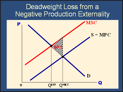
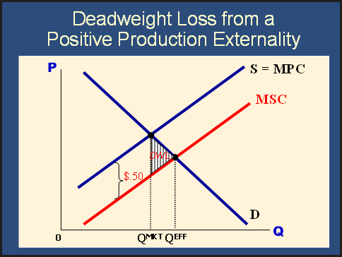
Because of this, a non-optimal amount of the good is produced and consumed. DWL is caused.

In general:

• Supply and Demand determine how much is produced.
• The social optimum is determined by Marginal Social Benefit and Marginal Social Costs.
• Because people are self-interested, supply and demand are determined by Marginal Private Benefit and Marginal Private Costs (ie S=MPC and D=MPB).
• Because Private and Social Benefits/Costs are different, the amount produced won’t be socially optimal.
• Because market mechanisms don’t supply the optimal amount (“a market failure”), there is a positive role for governments to play.

General Rules

Private Vs Social costs and benefits.

Costs

• The private costs represent the net costs to the producer of producing the good.
• The social costs represent all costs producing the good.
  • social cost = private costs of production + production externalities

Benefits

• The private benefits represent the net benefits to the consumer of consuming the good.
• The social benefits represent all benefits of consuming the good
  • social benefits = private benefits of consumption + consumption externalities

Which Curve do I shift?

With a Production externality, shift the Supply curve (because the supply curve represents production)

• This causes a difference between MPC and MSC.
• A negative production externality increases MSC above S=MPC.
• A positive production externality lowers MSC below S=MPC.

With a Consumption externality, shift the Demand curve (because the demand curve represents consumption)

• This causes a difference between MPB and MSB.
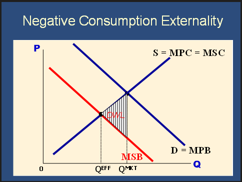
• A negative consumption externality lowers MSB below D=MPB.
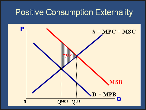
• A positive consumption externality raises MSB above D=MPB.

How do I find Market Quantity and Efficient Quantity?

The market quantity of carbon dioxide is determined by private costs and benefits. The efficient quantity is determined by social costs and benefits.

The market quantity is at the intersection of Supply/MPC and Demand/MPB

1. Private costs and benefits determine the amounts that people choose to produce and consume.
2. Use the original S and D curves to find the market quantity.
   1. MPB is the Demand curve
   2. MPC is the Supply curve

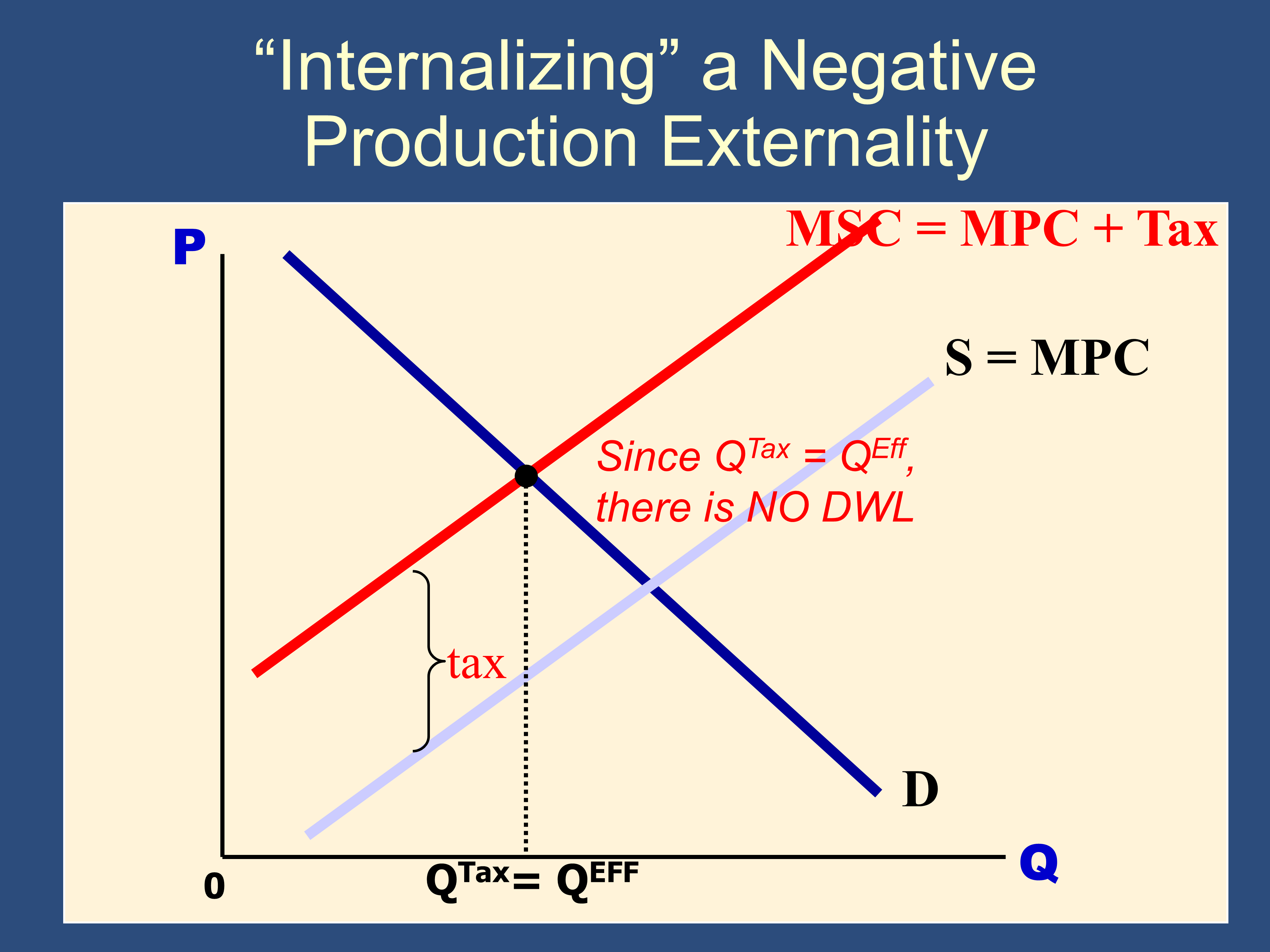
The efficient quantity is at the intersection of Marginal Social Costs and Marginal Social Benefits

1. Social costs and benefits determine the amounts that should be produced and consumed.
2. Use the shifted curves (if there are any) to find the efficient quantity.
   1. MSB is Demand curve, shifted by any external benefit/cost of consumption
   2. MSC is Supply curve, shifted by any external benefit/cost of production

Three Conditions for Perfect Competition

1. Many buyers and sellers ✔
   • Violations: Monopoly and Imperfect Competition
2. Well-specified property rights
   • Violations: Externalities
3. Complete information—well informed buyers and sellers
   • Violations: Asymmetric information

Production Externalities

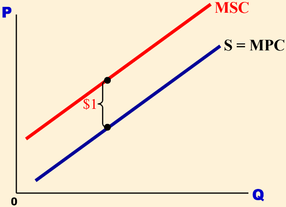
Negative Production Externality

Example: A polluting factory

$\text{Marginal Social Cost (MSC)} = \text{Marginal Private Cost (MPC)} + \text{Additional Cost to Society}$

$MSC > MPC$

Q	Marginal Private Cost (MPC)	Additional Cost to Society	Marginal Social Cost (MSC)
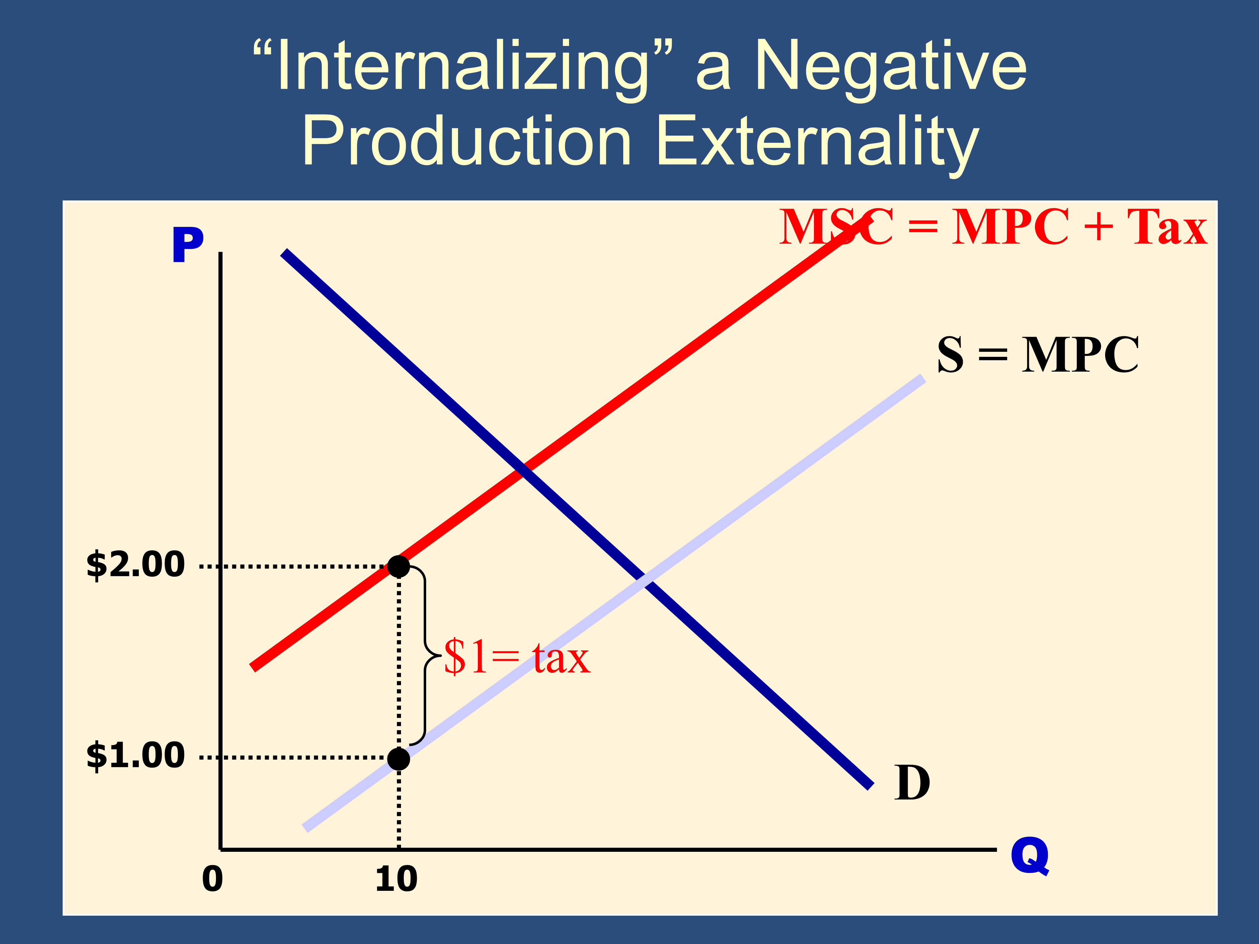
10	$1.00	$1.00	$2.00
15	$1.50	$1.00	$2.50
20	$2.00	$1.00	$3.00
25	$2.50	$1.00	$3.50
30	$3.00	$1.00	$4.00

MSC Curve Above MPC (or S) Curve
Supply curve shifts up.

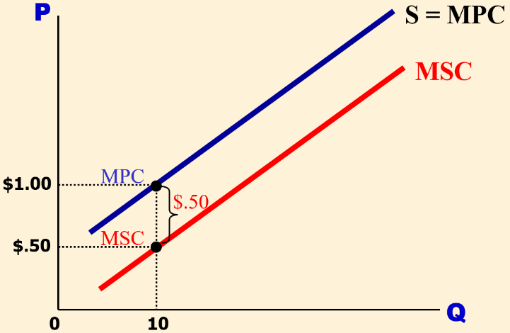
Positive Production Externality

Example: a university producing education has a byproduct of producing research. When you produce honey, you produce polinators for nearby plants.

$\text{Marginal Social Cost (MSC)} = \text{Marginal Private Cost (MPC)} - \text{Additional Benefit to Society}$

$MSC < MPC$

Q	MPC	Additional Benefit to Society	MSC
10	$1.00	$.50	$.50
15	$1.50	$.50	$1.00
20	$2.00	$.50	$1.50
25	$2.50	$.50	$2.00
30	$3.00	$.50	$2.50

MSC Curve Below MPC (or S) Curve
Supply curve shifts down

Consumption Externalities

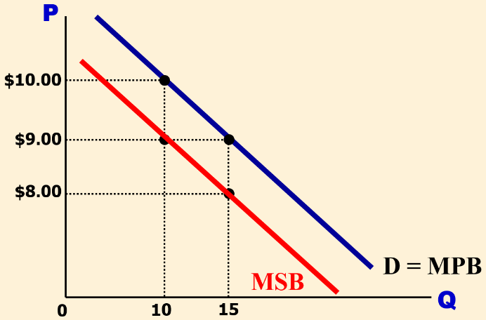
Negative Consumption Externalities

Example: Consumption of loud music. Second hand smoke. Squeaky shoes that make a student’s dogs bark. Alcohol.

$MSB < MPB$

Q	MPB	Additional Cost to Society	MSB
10	$10.00	$1.00	$9.00
15	$9.00	$1.00	$8.00
20	$8.00	$1.00	$7.00
25	$7.00	$1.00	$6.00
30	$6.00	$1.00	$5.00

MSB Curve Below MPB (or D) Curve
Demand curve shifts Down

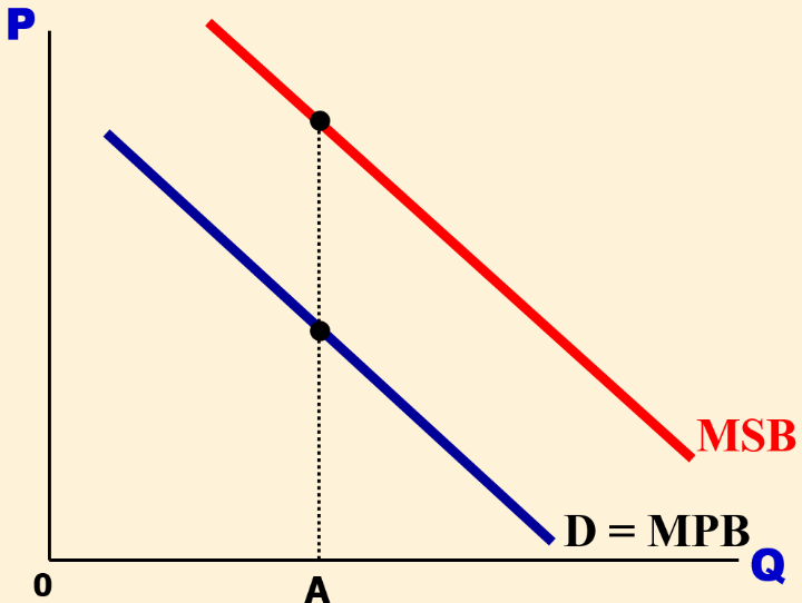
Positive Consumption Externalities

Example: when you consume education, you become a better voter. When you consume yoga, you become kinder to the people around you.

$MSB > MPB$

Q	MPB	Additional Benefit to Society	MSB
10	$10.00	$1.00	$11.00
15	$9.00	$1.00	$10.00
20	$8.00	$1.00	$9.00
25	$7.00	$1.00	$8.00
30	$6.00	$1.00	$7.00

MSB Curve Above MPB (or D) Curve
Demand curve shifts Up

Summary

	Production	Consumption
Negative	$MSC > MPC$ MSC Curve Above MPC (or S) Curve $Q^{EFF} < Q^{MKT}$	$MSB < MPB$ MSB Curve Below MPB (or D) Curve $Q^{EFF} < Q^{MKT}$
Positive	$MSC < MPC$ MSC Curve Below MPC (or S) Curve $Q^{EFF} > Q^{MKT}$	$MSB > MPB$ MSB Curve Above MPB (or D) Curve $Q^{EFF} > Q^{MKT}$

If there is no consumption externality, then MSB=MPB (ie the demand curve).
If there is no production externality, then MSC=MPC (ie the supply curve).

No Externalities	$MSC = MPC$ $MSB = MPB$
Just a positive or negative production externality	$MSC \neq MPC$ (ie $MSC < MPC$ or $MPC < MSC$) $MPB = MSB$
Just a positive or negative Consumption Externality	$MPB \neq MSB$ (ie $MPB > MSB$ or $MPB < MSB$)
BOTH a production externality AND a consumption externality	$MSC \neq MPC$ $MSB \neq MPB$

Market Quantity: S=MPC and D=MPB
Efficient Quantity (Omniscient Planner cares about everyone): MSC and MSB
DWL is between the Market Quantity and the Efficient Quantity.
Economists try to care about everyone, so DWL is between MSC and MSB

Combining all of the above informatin into one enormous table, we get the following (shared by a student):

Type of Externality	$Q_\text{market}$	$Q_\text{efficient}$	Which curve shifts?	Outcome
Negative Production Externality	$MPC = MPB$ ($MPB = \text{Demand}$)	$MSC = MSB$ ($MSB = \text{Demand}$)	$MSC > MPC$	$Q_\text{market} > Q_\text{efficient}$ → Overproduction/Overconsumption
Positive Production Externality	$MPC = MPB$ ($MPB = \text{Demand}$)	$MSC = MSB$ ($MSB = \text{Demand}$)	$MSC < MPC$	$Q_\text{market} < Q_\text{efficient}$ → Underproduction/Underconsumption
Negative Consumption Externality	$MPB = MPC$ ($MPC = \text{Supply}$)	$MSB = MSC$ ($MSC = \text{Supply}$)	$MSB < MPB$	$Q_\text{market} > Q_\text{efficient}$ → Overproduction/Overconsumption
Positive Consumption Externality	$MPB = MPC$ ($MPC = \text{Supply}$)	$MSB = MSC$ ($MSC = \text{Supply}$)	$MSB > MPB$	$Q_\text{market} < Q_\text{efficient}$ → Underproduction/Underconsumption
Insights from this column	$Q_\text{market}$ is always where $MPB = MPC$.	$Q_\text{efficient}$ is always where $MSB = MSC$.	Production Ext: shift Supply=MPC to get MSC. Consumption Ext: shift Demand=MPB to get MSB.	With negative externalities, we make too much, so $Q_\text{market} > Q_\text{efficient}$ With positive externalities, we make too little, so $Q_\text{market} < Q_\text{efficient}$.

Private Solutions to Externalities

Government action is not always needed to solve the problem of externalities.
Types of Private Solutions:

• Moral codes and social sanctions
• Contracting between parties

The Coase theorem is a proposition that if private parties can bargain without cost over the allocation of resources, they can solve the problem of externalities on their own.

• Transaction costs are the costs that parties incur in the process of agreeing to and following through on a bargain
• Sometimes the private solution approach fails because transaction costs can be so high that private agreement is not possible.

Public Policies Toward Externalities

When externalities are significant and private solutions are not found, government may attempt to solve the problem through …

• command-and-control policies.
• market-based policies

Command-and-Control Policies: Regulation
Usually take the form of regulations:

• Forbid certain behaviors.
• Require certain behaviors.

Examples:

• Requirements that all students be immunized.
• Stipulations on pollution emission levels set by the Environmental Protection Agency (EPA).

Market-Based Policies: Corrective Taxes

• Government uses taxes to align private incentives with social efficiency.
• Corrective taxes are taxes enacted to correct the effects of a negative externality.
  • Also called Pigovian taxes, first proposed by: Arthur Cecil Pigou (1877 – 1959)

Examples of Regulation versus Corrective Tax: If the EPA decides it wants to reduce the amount of pollution coming from a specific plant. The EPA could…

• tell the firm to reduce its pollution by a specific amount (i.e. regulation).
• levy a tax of a given amount for each unit of pollution the firm emits (i.e. corrective tax).