👨‍🏫 Notes on Lecture 6

Pindyck and Rubinfeld: Sections 8.1 - 8.5
See also: 🔎 Market Structure Comparison

Perfect Competition

Three Preconditions for Perfect Competition:

1. Many buyers and sellers (no monopoly; no strategic interaction/game theory)
2. Complete information (no asymmetric information)
3. Well-specified property rights (no externalities)

Characteristics of Perfectly Competitive Firm

• Homogenous products
• Ease of entry and exit
• Price-taking behavior

Short Run Profit Maximization Condition

• For continuous quantities, produce that $q^*$ for which $P = MR = MC$ (derived from calculus)

  • Continuous goods can be subdivided, like gasoline or gold

• For discrete quantities, produce the highest q for which $P = MR \geq MC$

  • Discrete goods can’t be subdivided, like cars or cell phones

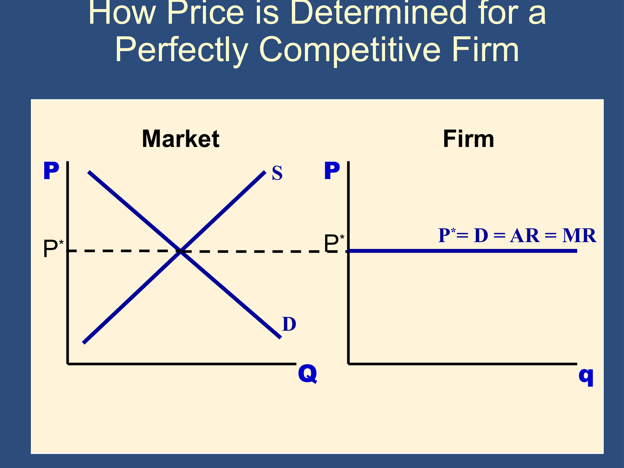
Market Supply and demand determine $P^*$ and firms are price takers.

Profit and Long Run vs Short

Short Run: some factors of production are fixed. (Therefore, you have fixed costs)
Long Run: all factors of production are variable. (Therefore, all costs are variable, not fixed)

Example:

• Suppose you have a lease and employees.
• You can lay off or furlough workers (variable factor of production).
• But you are still contractually obligated to pay the lease (fixed factor of production in the SR).
• SR ends and LR begins in this example when the lease ends. The lease becomes variable because you don’t have to renew.
• In short run, you can shut down, but you still have to pay lease. In long run, you can exit and have no expenses or revenue.

Profit, Shut Down, and Exit

• $\text{Profit} = TR - TC = q^*(P - AC)$
  • Therefore: $P > AC$ ⇨ $\text{profit} > 0$! $P = AC$ ⇨ $\text{profit} = 0$. $P < AC$ ⇨ $\text{profits} < 0$ (losses; want to exit).
• (Short Run) Shut Down: $AVC > P$
• (Long Run) Exit: $AC > P$

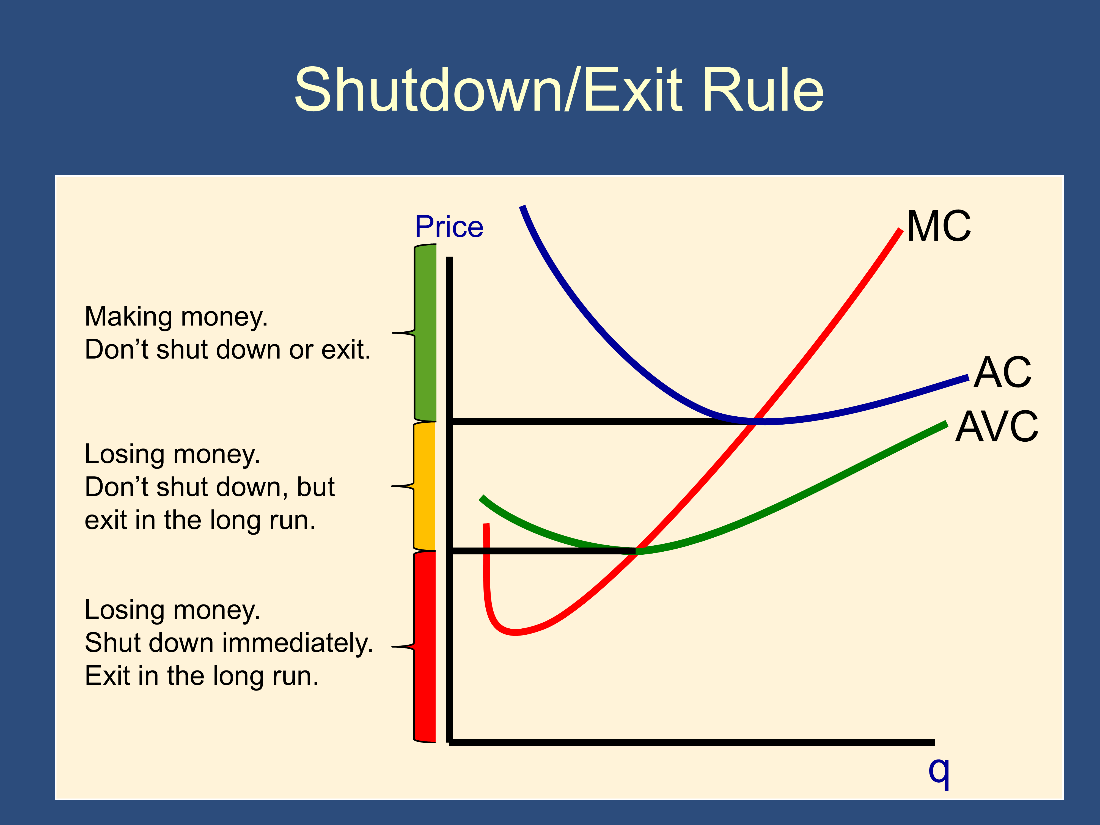
Shut Down happens in short run when $P < AVC$. Must still pay FC.
Exit happens in the long run, when $P < AC$. In the long run, FC become variable and can be avoided.

Three steps to solve a perfect competition problem

Step 1: $P = MC$ to figure out $q^*$
 (Or, for discrete good, choose largest q where $P \geq MC$.)
Step 2: Do you shut down ($P < AVC$) or, in LR, exit ($P < ATC$)? (always check whether you would stay in business or not)
Step 3: Wrap up ($\text{profit} = q(P - AC)$) You apply the same three steps on a diagram, table, or with algebra.

Diagram example with the 3 steps:

Note: $P > AC$, so can make a profit. Won’t shut down!

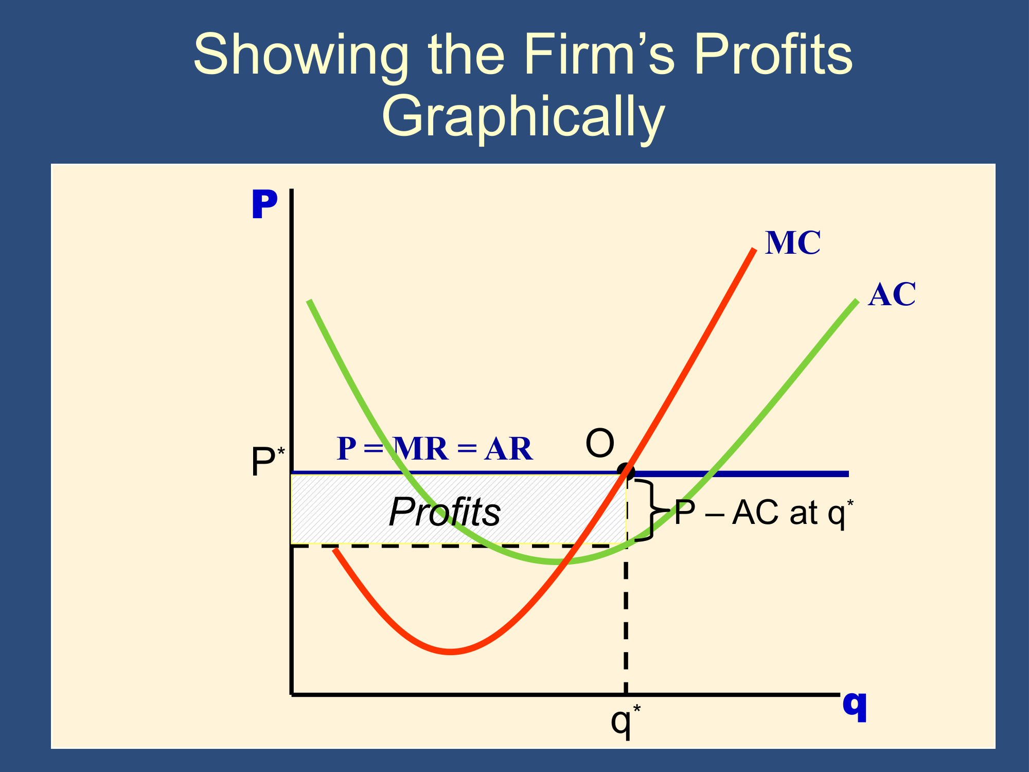
✏️ suppose $P^* = \$9$, $q^* = 800$, and the additional point is as labeled above.

✔ Click here to view answer

Step 1: $P = MC$ (or $P \geq MC$) to figure out $q^*$

• The intersection of the price line and the MC curve occurs at point O. This corresponds with a quantity of $q^*$

Step 2: Do you shut down ($P < AVC$) or, in LR, exit ($P < ATC$)? (always check whether you would stay in business or not)

• *AC is always higher than AVC, because $AC = AVC + AFC$. The diagram shows that P is higher than AC, so P is definitely higher than AVC. When $P > AVC$, we don’t shut down.
• Therefore, we produce $q = q^*$. $q^*$ is the optimal quantity to produce if you don’t shut down. When I write $q = q^*$ it means that I’m actually producing $q^*$.*

Step 3: Wrap up ($\text{profit} = q(P - AC)$)

• Now that we have determined q, we can look up AC. AC could be very high or very low, but for our company, right now, $AC = \$7$.
• $\text{profit} = q^*(P - AC) = 800 \times (\$9 - \$7) = \$1{,}600 \quad\text{✅}$

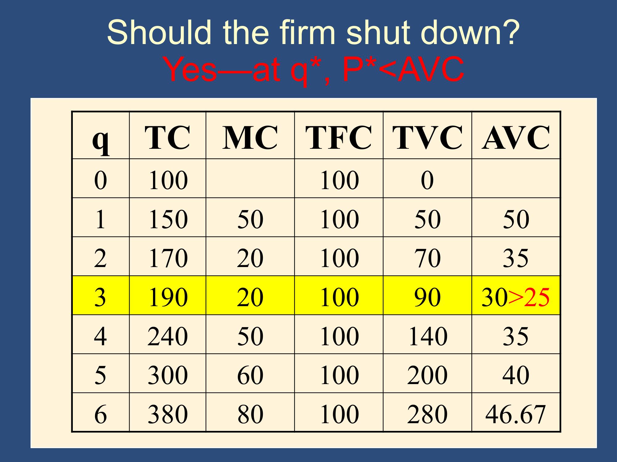
Table example with the 3 steps:

Suppose $P = \$25$. This table represents a discrete good, so we choose the largest $q^*$ where $P \geq MC$. This happens at $q^* = 3$. We shut down because when we produce $q^* = 3$ units, $P^* < AVC$ ($\$25 < \$30$).

Algebraic example with the 3 steps:

Suppose $MC = 200 + 3q$, $P = 410$, and $AC = 200 + 1.5q$ and that the firm produces positive output (ie $q > 0$). What is profit?
Step 1: Set $P = MC$ and solve for $q^*$: (we won’t give your algebra problems with discrete goods, so you can assume it is continuous and use $P = MC$, not $P \geq MC$)

• $410 = 200 + 3q$
• $210 = 3q$ (subtract 200 from both sides to get rid of the 200)
• $q^* = 70$

Step 2: we are told the firm produces positive output, so we know it doesn’t shut down.
Step 3: $AC = 200 + 1.5q = 200 + 1.5 \times 70 = 305$
$\text{Profit} = q^*(P - AC) = 70 \times (\$410 - \$305) = \$7{,}350$

Long Run

The main picture of Long Run perfect competition
At the “triple intersection,” $P = AC$, so $\text{profits} = q(P - AC) = 0$.

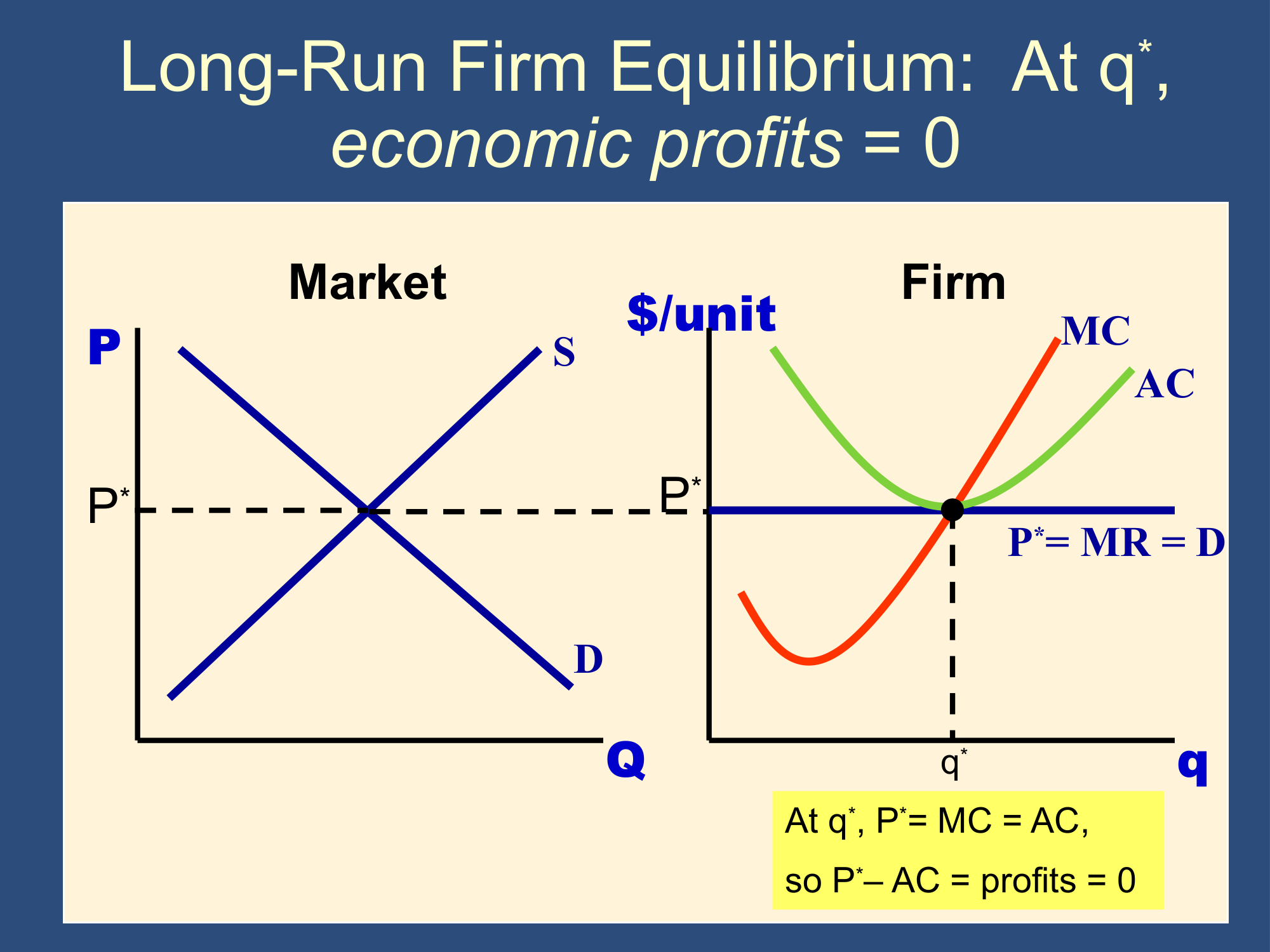
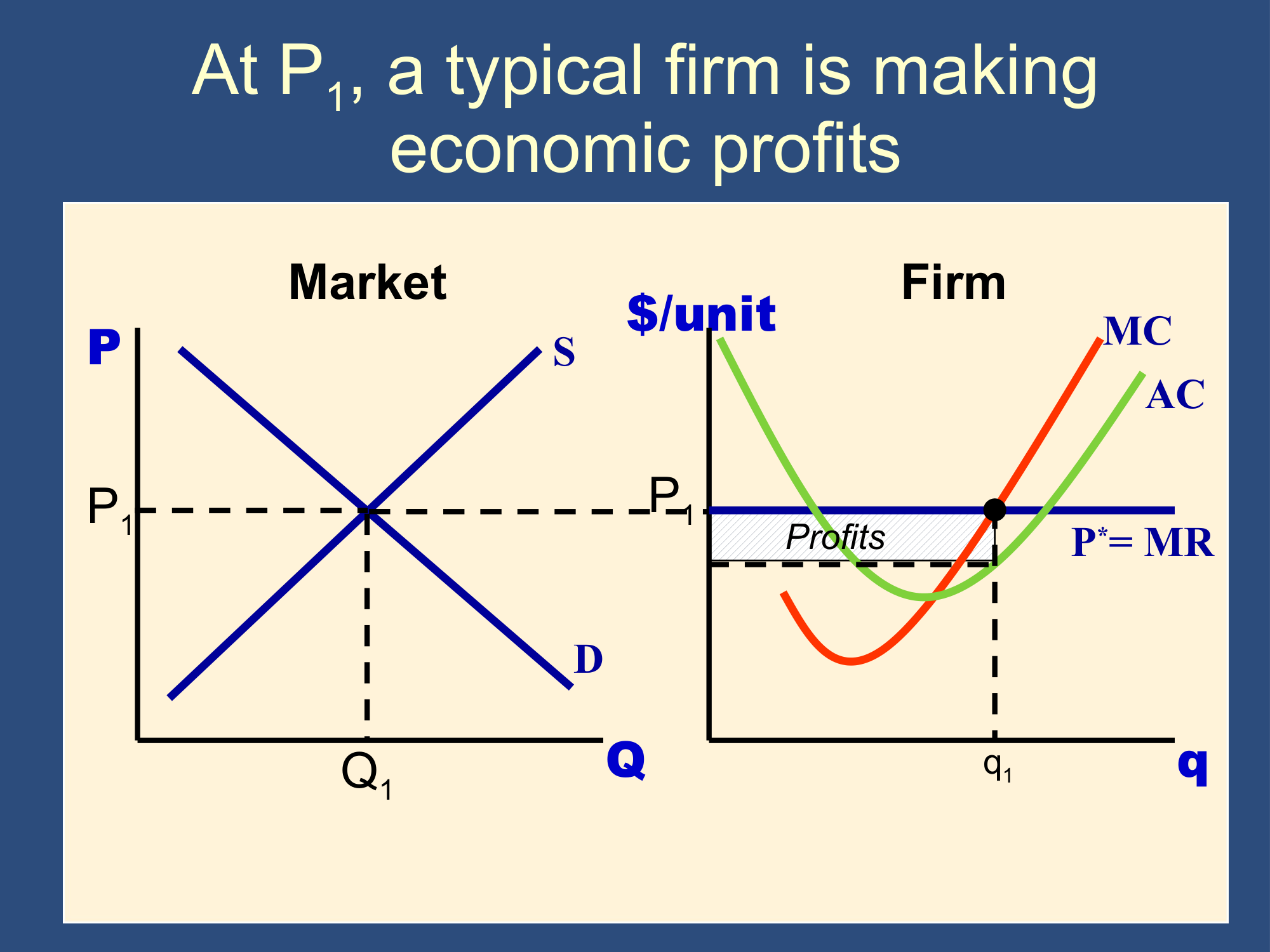
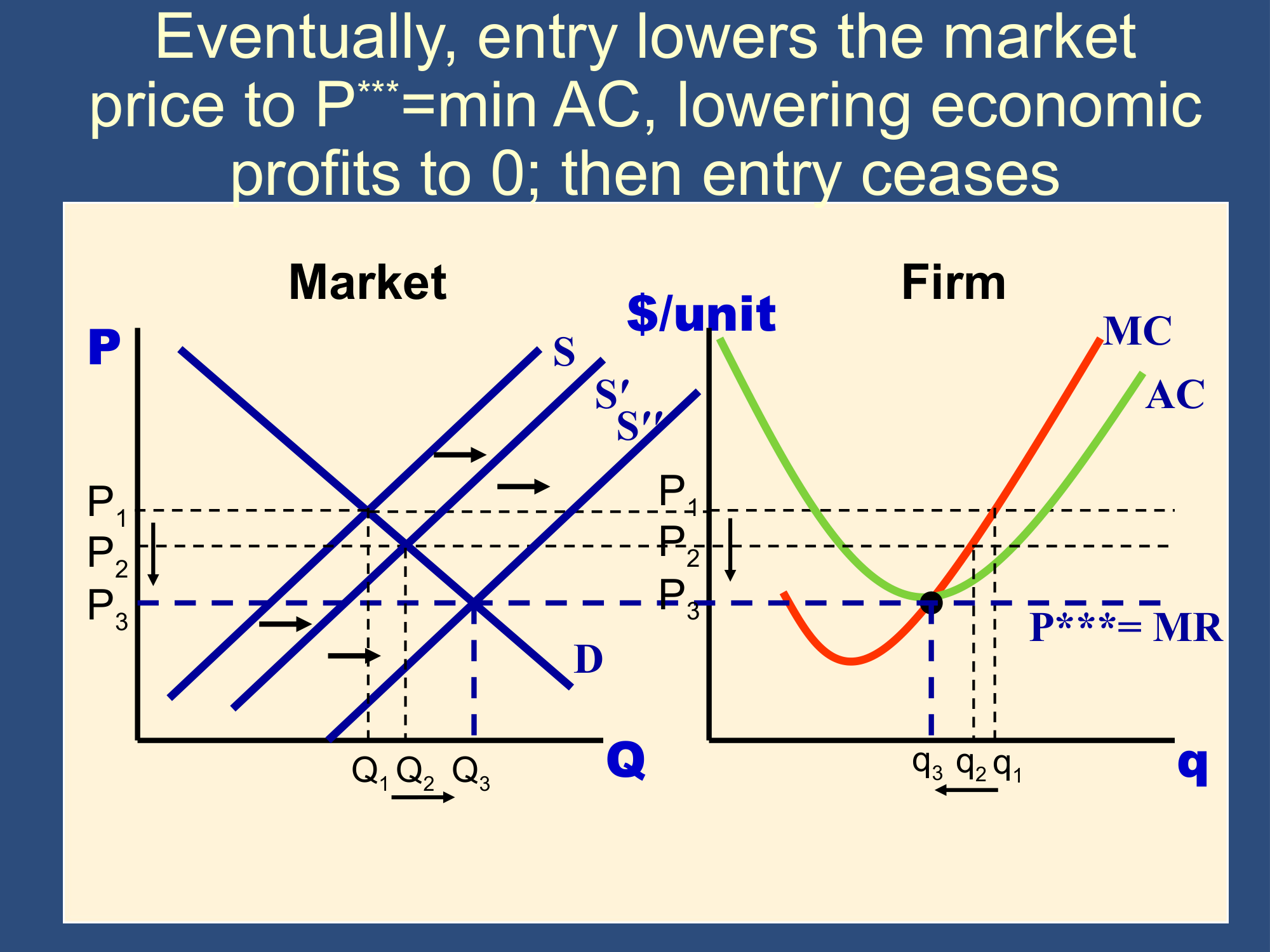
Why are profits always zero ($\pi = 0$) in the long run?

$\pi > 0$ → Entry occurs → Number of firms ↑
 → Supply ↑ → Supply curve shifts Right
 → $P^*$ ↓, $Q^*$ ↑, $\pi$ ↓
 → process continues until $\pi = 0$

If you make positive profit, then entry will occur until your profit declines, eventually declining down to zero.

	→

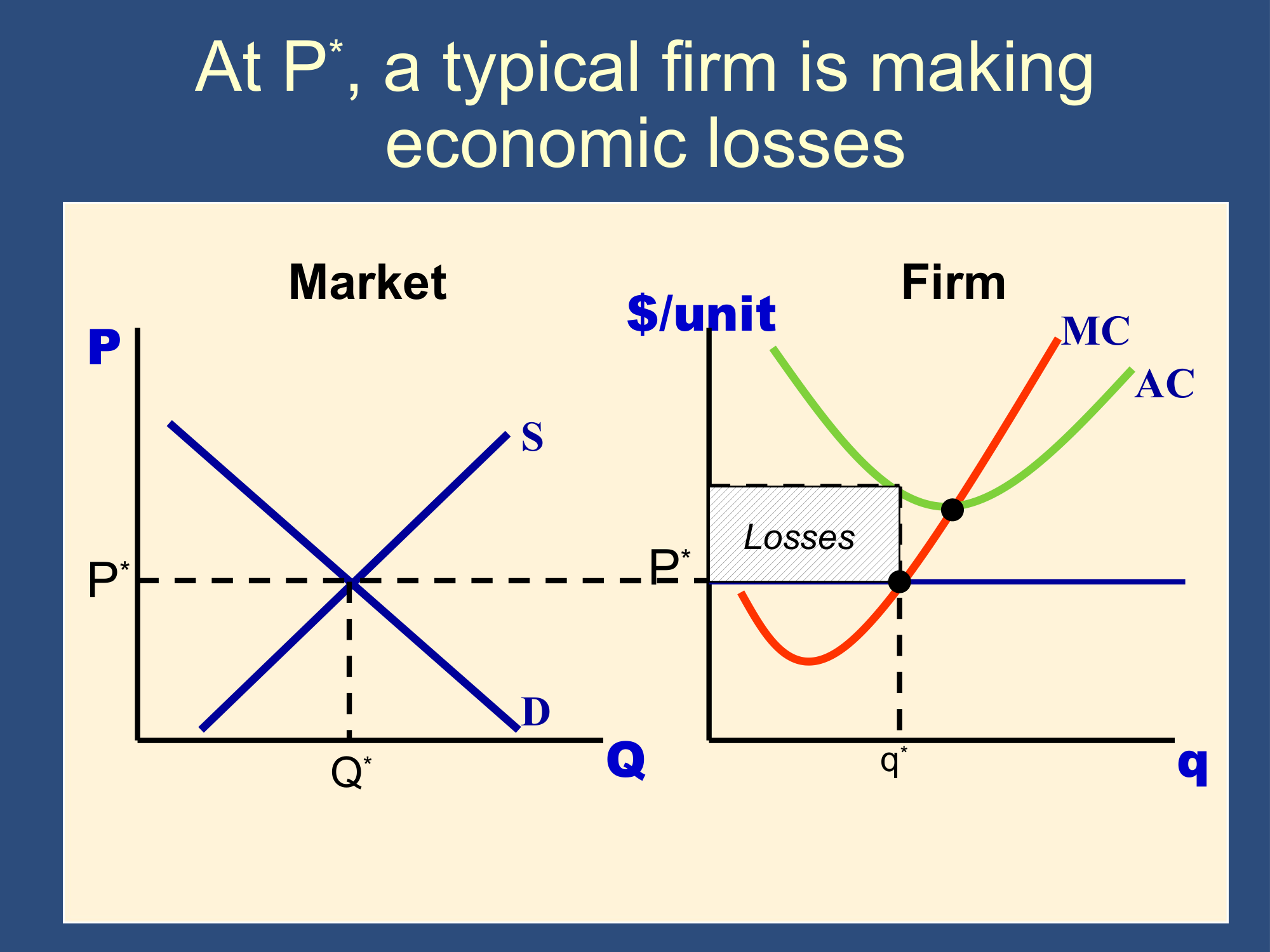
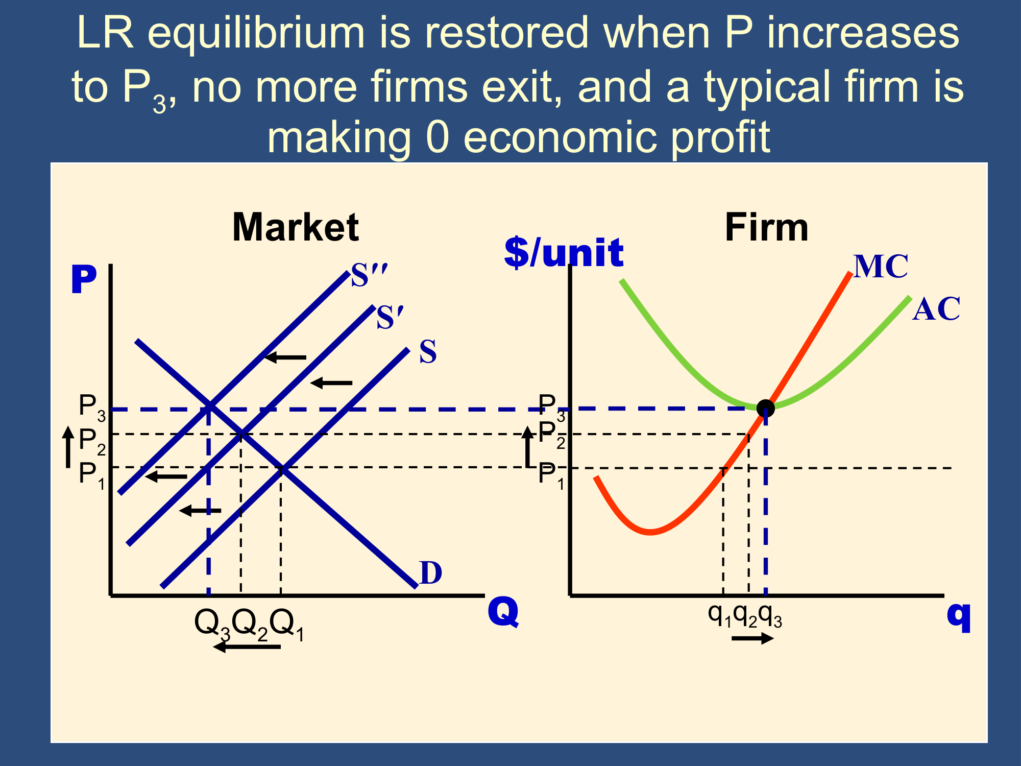
$\pi < 0$ → Exit occurs → Number of firms ↓
 → Supply ↓ → Supply curve shifts L
 → $P^*$ ↑, $Q^*$ ↓, $\pi$ ↑
 → process continues until $\pi = 0$

If you losing money, then exit will occur until the remaining firms lose less money. The process will continue until firms aren’t losing any money at all (ie $\text{profit} = 0$).

	→

Accounting vs. Economic Profits

Explicit costs are costs where money is spent.
Implicit costs are nonmonetary costs, like effort or using a fixed resource that is already owned.

$\text{Accounting Costs} = \text{Explicit costs only}$
$\text{Economic Costs} = \text{Explicit} + \text{Implicit costs}$
Clearly, $\text{Economic Costs} > \text{Accounting Costs}$, because Economic costs include Implicit costs.

$\text{Accounting Profit} = \text{Revenue} - \text{Accounting Costs}$
$\text{Economic Profit} = \text{Revenue} - \text{Economic Costs}$
Because Economic costs are larger, Economic Profit must be smaller. Therefore, a firm can have accounting profits even when economic profit is zero (which it will be in the long run if there is free entry).