👨‍🏫 Notes on Lecture 2

Basic definitions

• Utility = happiness, satisfaction or well-being
• Marginal Utility (MU) = the additional utility you get from one additional unit of a good or service
• $MU_X = \frac{ΔU}{ΔX}$
• Diminishing Marginal Utility: When I don’t have much of good X, MUX is high. When I am already consuming a lot of good X, MUX is low. Most goods have diminishing marginal utility.

Indifference Curves

Indifference curves are like contours on contour maps. Contour lines tell you how high you are on a mountain and indifference curves tell you how high you are in terms of happiness.

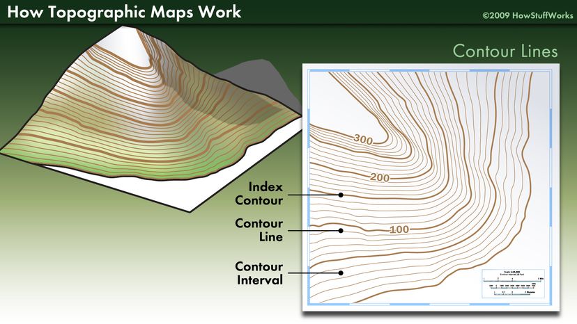
Image Credit: HowStuffWorks

There are four Principles of Indifference Curves

1. Higher indifference curves represent higher utility
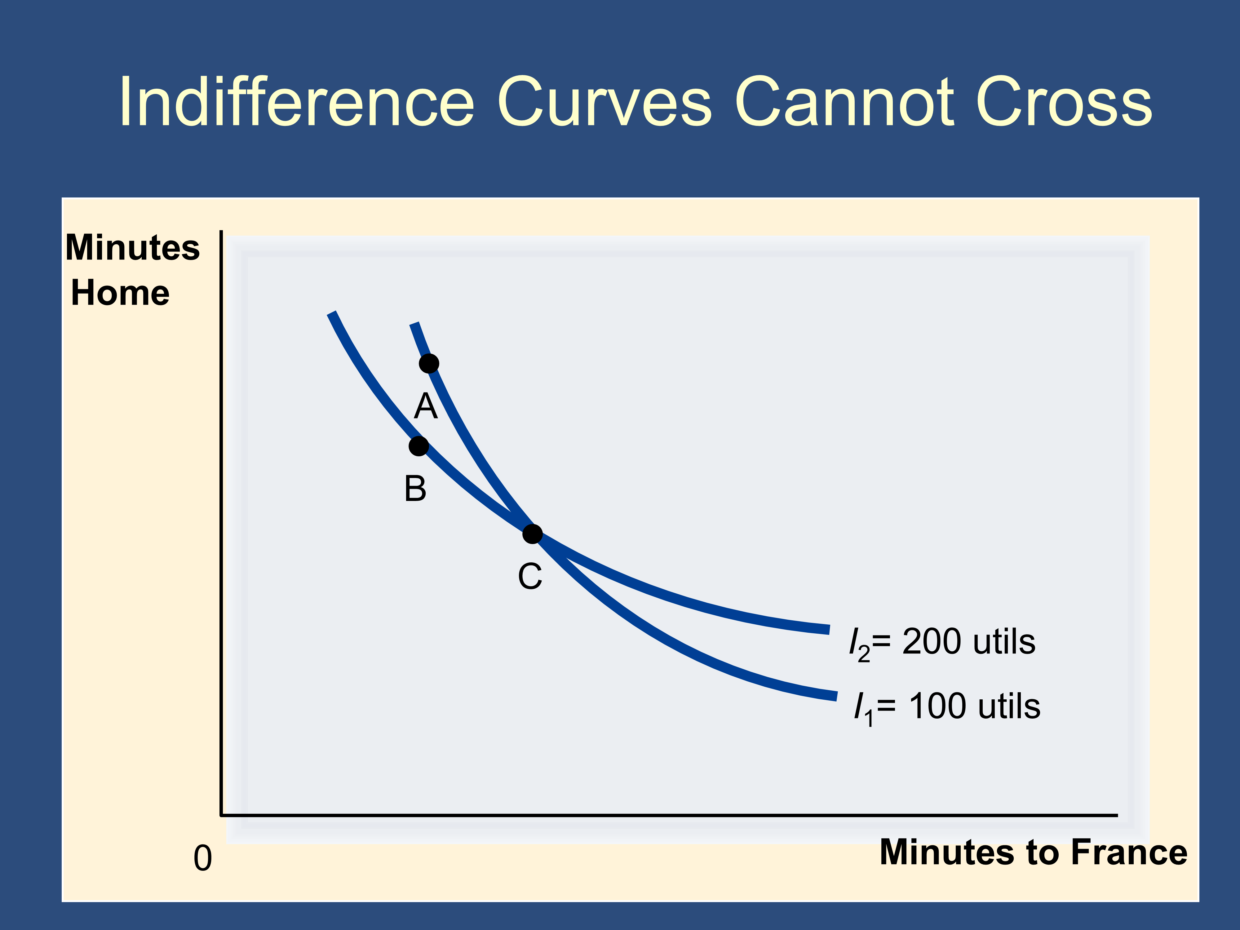
2. Indifference curves never cross (if they did, which IC would you be on at the intersection?)
3. Indifference curves cannot cross:
4. Indifference curves usually slope downward (if both goods are things you want to consume - ie if “both goods are good”)
5. Indifference curves are usually convex - bowed inward toward the origin (sometimes called “concave up”) (see MRS, below, for an explanation).

Marginal Rate of Substitution

For a more detailed presentation of the same ideas see: 🔎 Learning the MRS

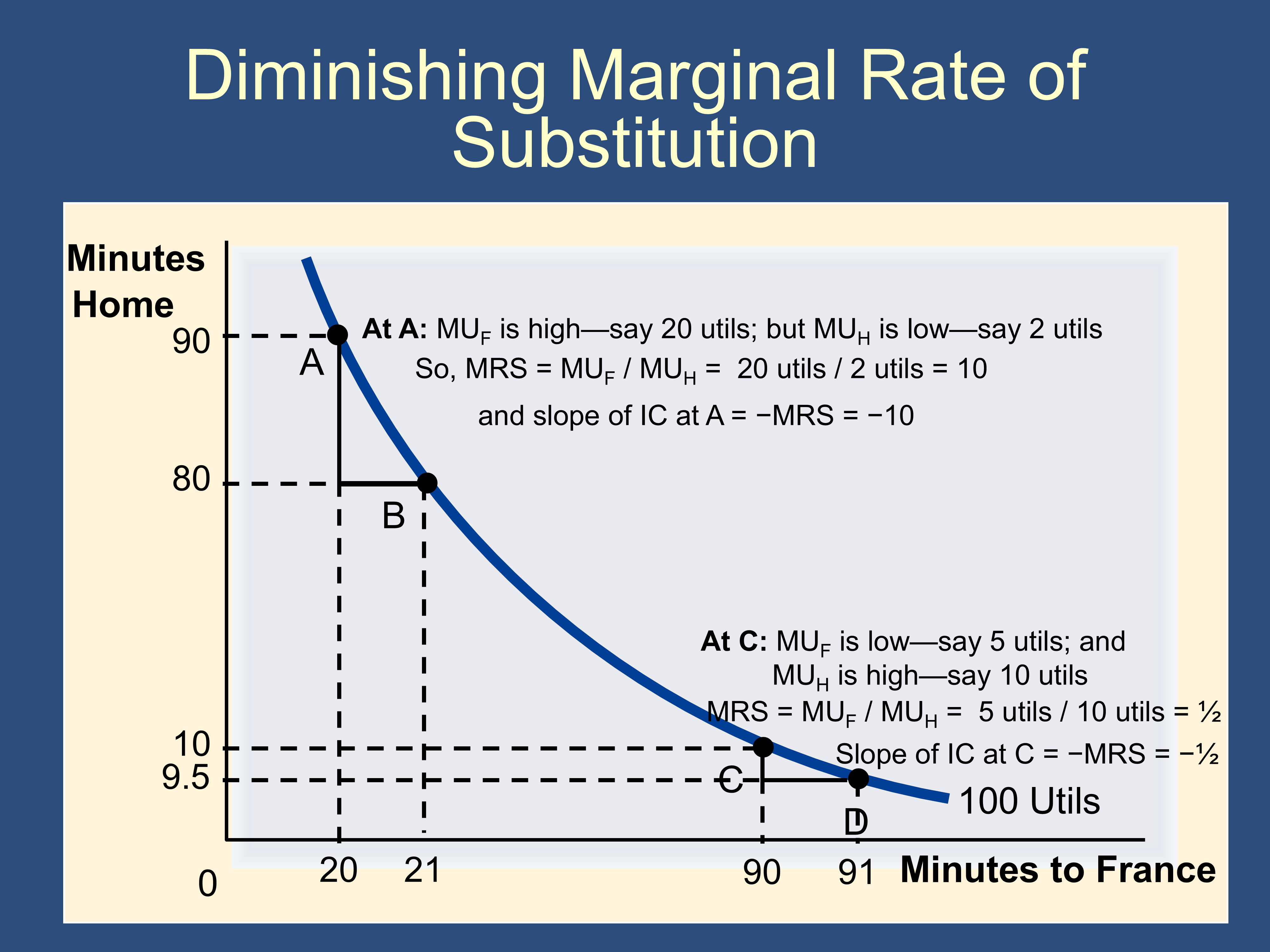
1. Marginal Rate of Substitution (MRS of X for Y) is the amount of good Y you are willing to give up to get one more unit of X. If you value X more than Y, you will give up more units of Y to get an additional unit of X
   • MRS measures the marginal value of one more unit of X…that value being measured in units of Y
2. $MRS=\frac{MU_X}{MU_Y}$ (Recall that the MU of a good declines as you consume more of it.)
   • Intuitively, if MU_X is high, I’ll give up many units of Y to get one more unit of X, so I would expect the MRS to be high. The above formula tells us that when MUx is high, MRS is also high.
   • Intuitively, if MU_Y is high, then the MRS should be low.
3. Diminishing Marginal Rate of Substitution means that as you move down along an indifference curve, MRS decreases (in other words, the IC gets flatter, as you move down along it).

Slope of the IC

Slope of IC = $-MRS = -\frac{MU_X}{MU_Y}$

Budget Constraints

Budget Constraints are easy if you just remember how to calculate the endpoints.

• If you purchase only good X, you can purchase a maximum of $\frac{B}{P_X}$.

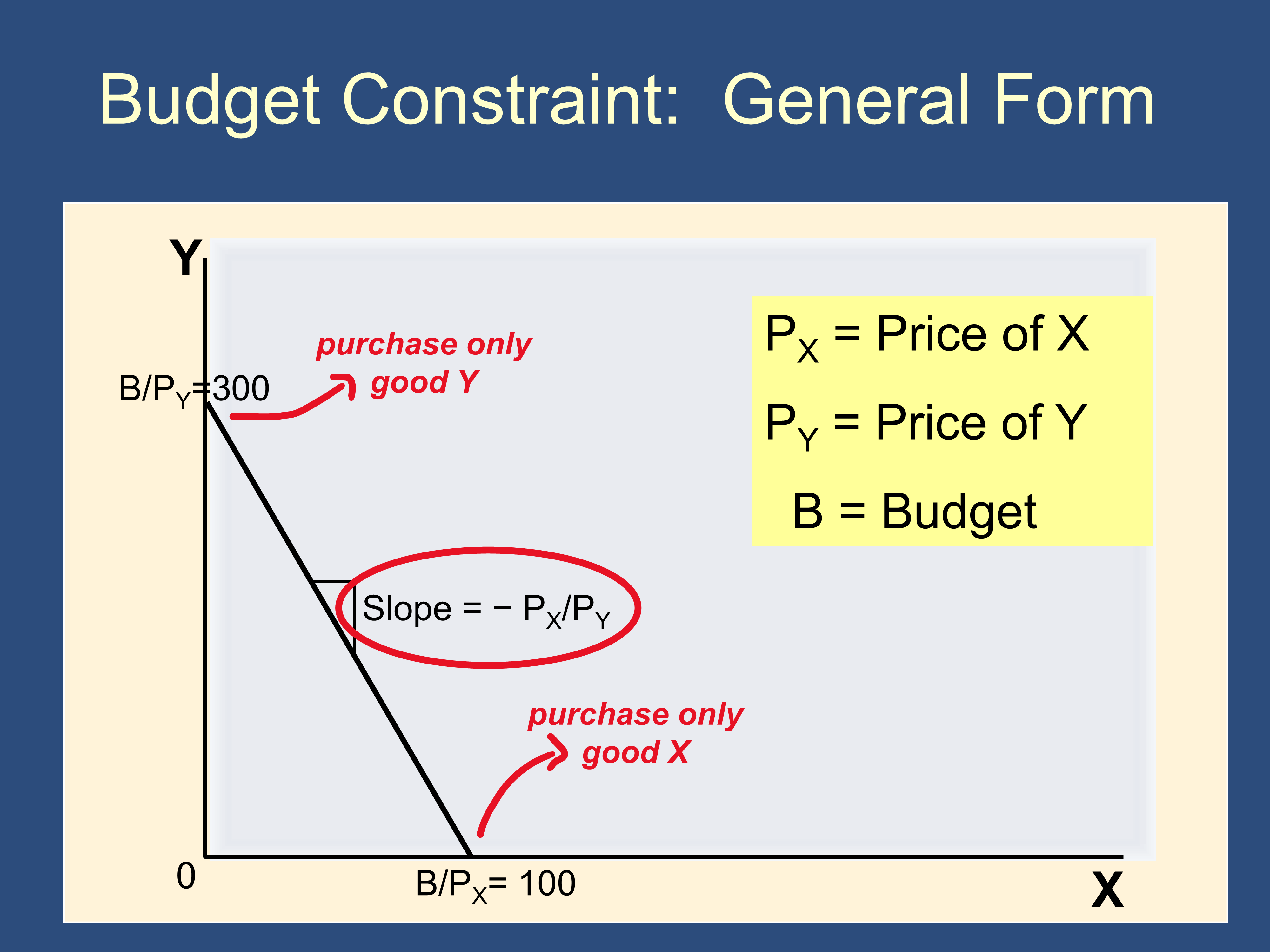
Recipe to draw a budget constraint:

1. Plot the point where you spend all your money on good Y (ie the point at $\frac{B}{P_Y}$ on the Y axis)
2. Plot the point where you spend all your money on good X (ie the point at $\frac{B}{P_X}$ on the X axis)
3. Draw a line connecting those two points. That is the BC.

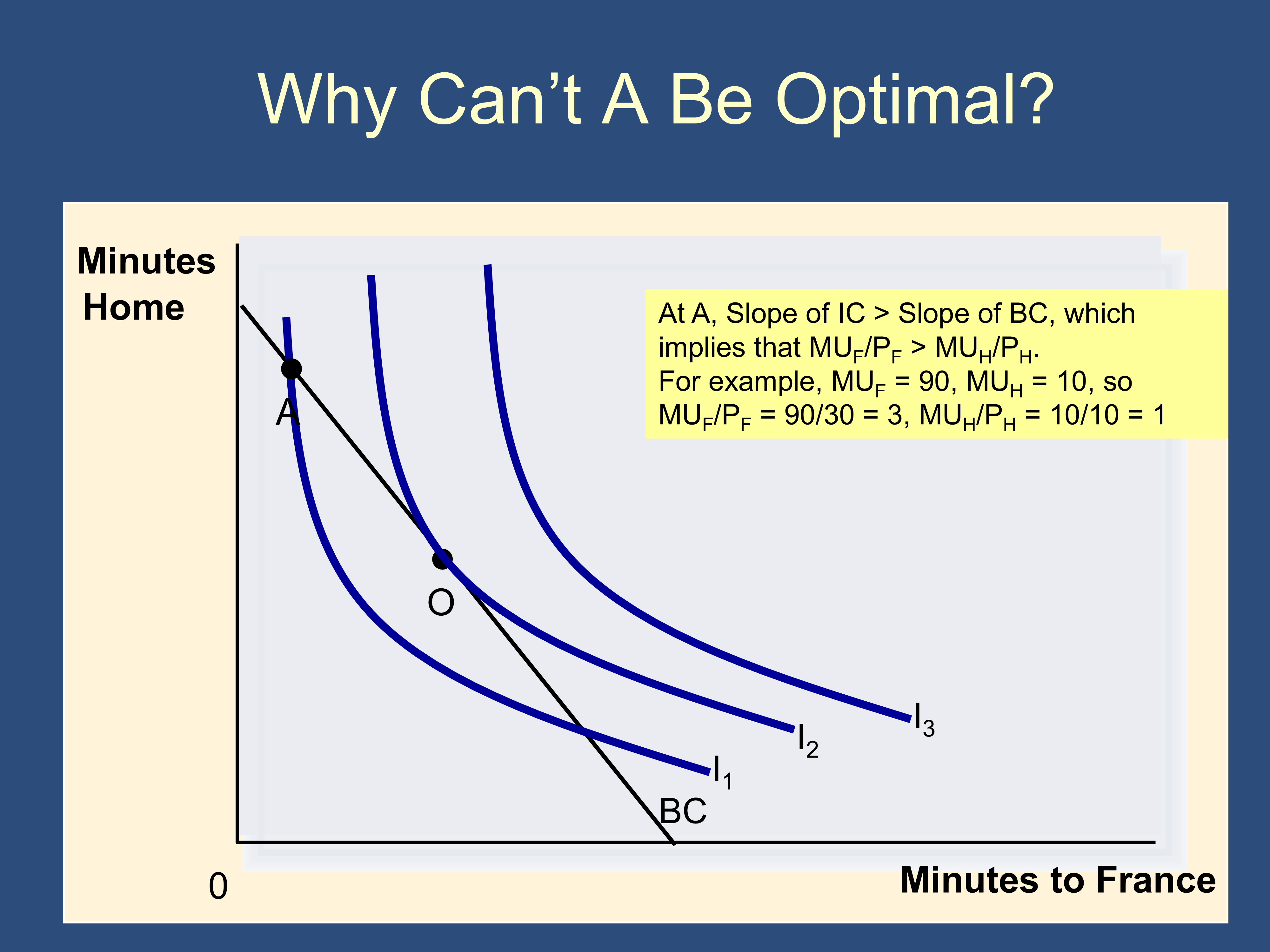
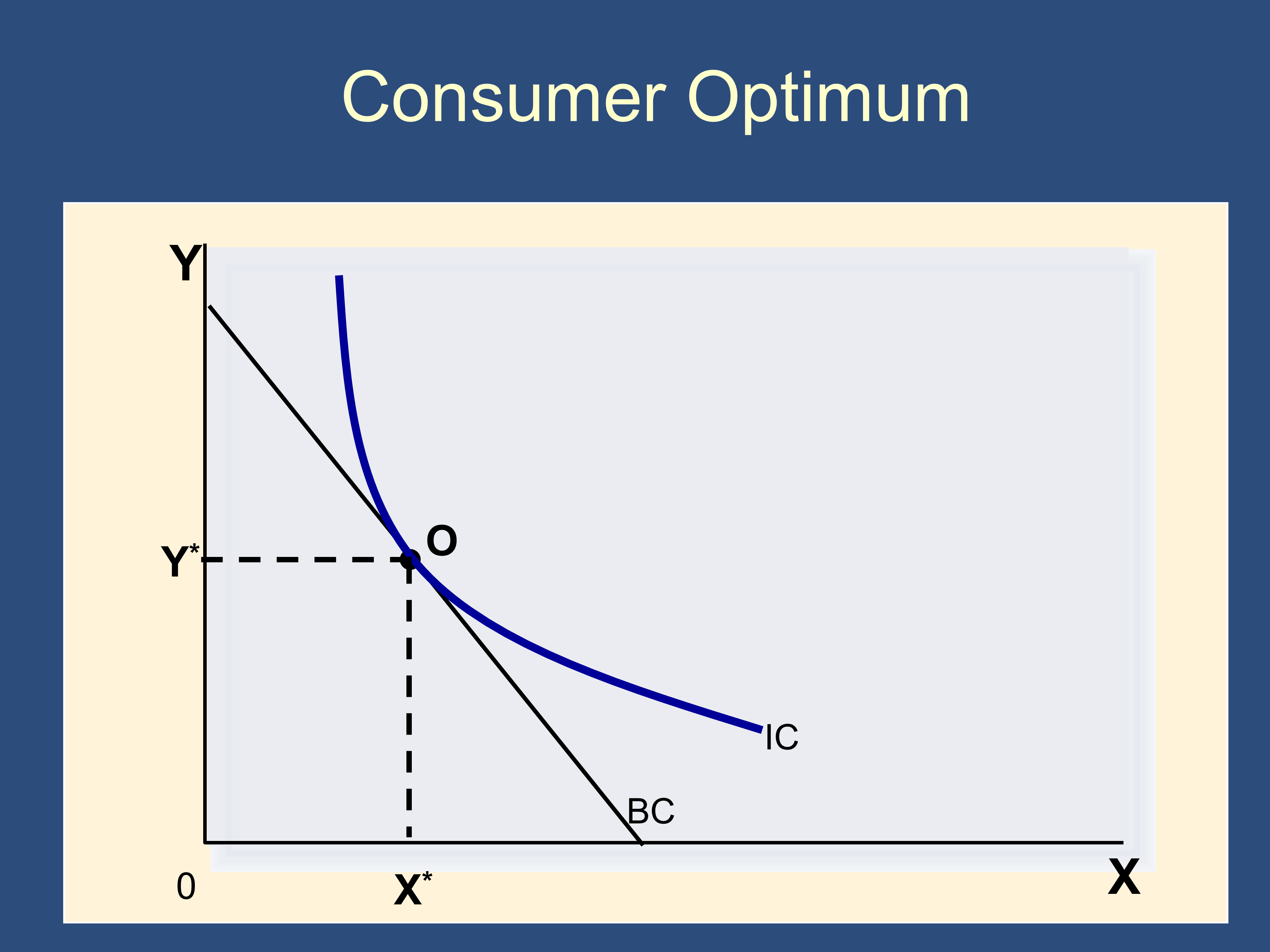
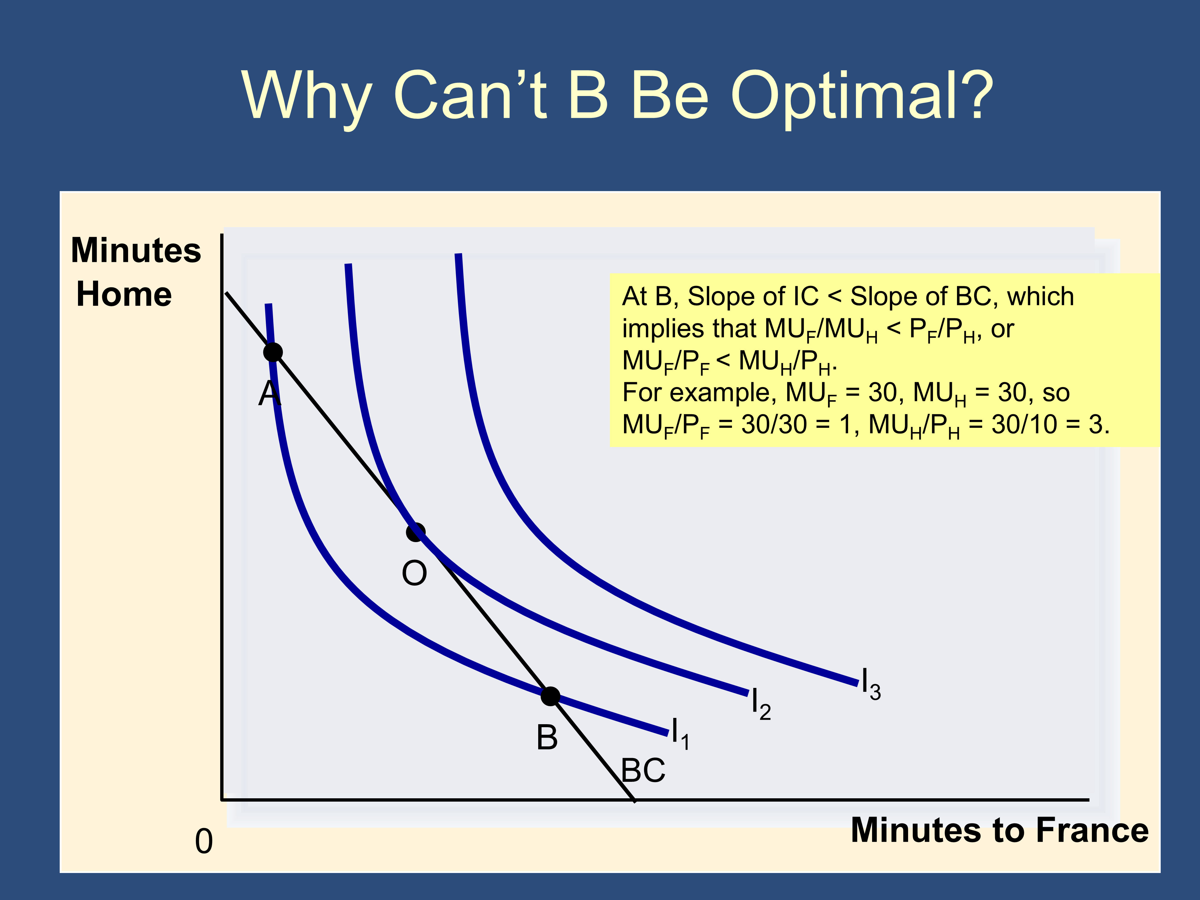
Optimization = Indifference Curves + Budget Constraints

The main optimization condition is just that the Slope of the IC = Slope of the BC

Three bears:

Too Much Y	Just Right	Too Much X

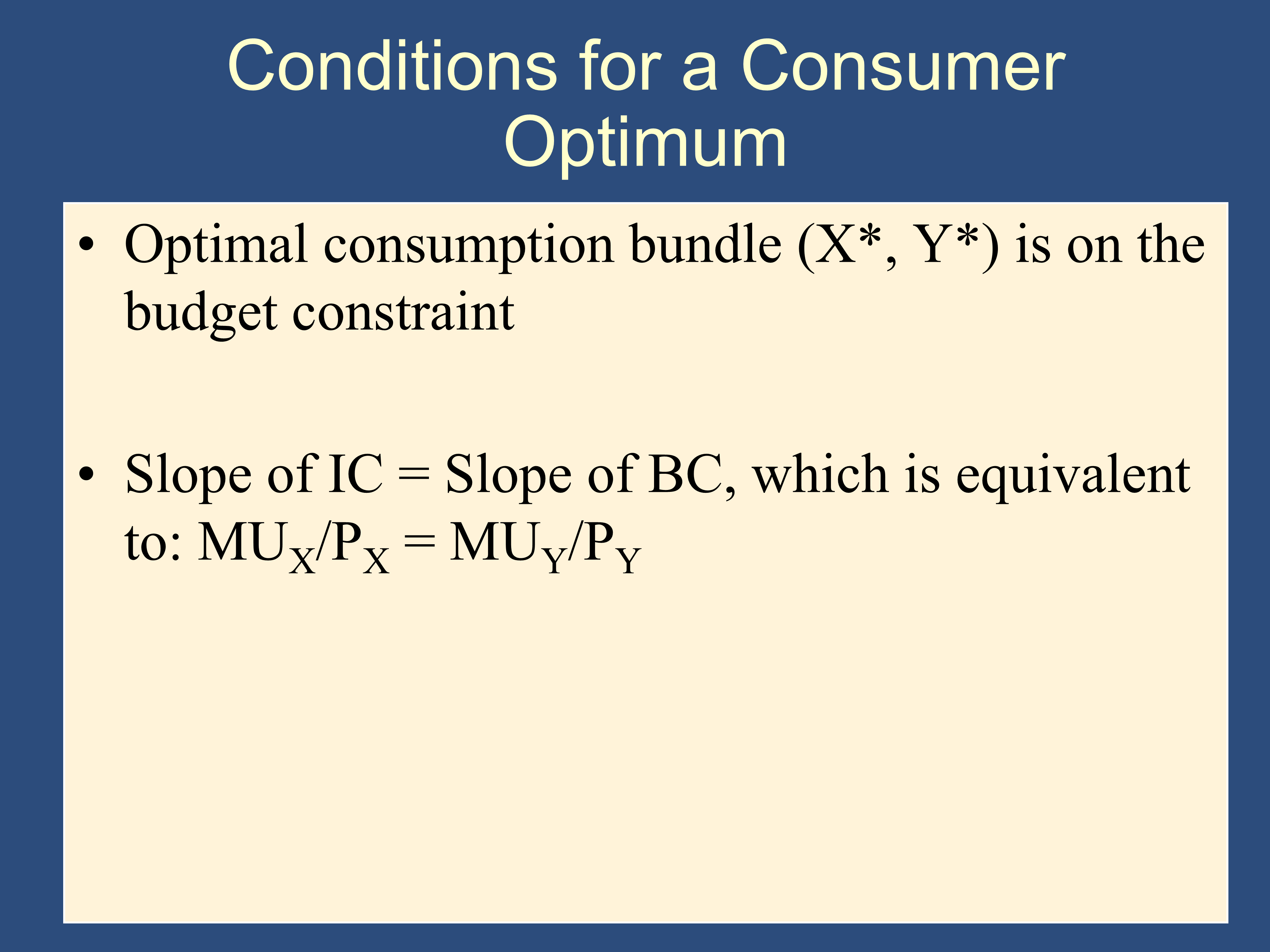
Conditions for a Consumer Optimum

Someone is buying the optimal goods (optimizing) if

1. they spend all of their money and
2. the “bang for the buck” of both goods are equal

Bruce presents this on the following slide:

However, in earlier slides, he introduces alternate versions of each of the two conditions for a consumer optimum. These alternate versions are important when solving problem, so you may find the following extended cheat sheet helpful:

First Condition for a Consumer Optimum:  a) Your optimal consumption bundle (X*,Y*) should be on the Budget Constraint. In other words, you must use all of your money. Alternate Version:  b) $X^∗×P_X +Y^∗×P_Y = B$

Second Condition for a Consumer Optimum:  a) Slope of IC = Slope of BC  b) $\frac{MU_x}{P_x} = \frac{MU_y}{P_y}$ ("Bang for the buck" formulation) This ensures that you spend your money on the things that bring you the most utility per dollar. Alternate versions:  c) $MRS=\frac{P_x}{P_y}$  d) Ratio of MUs: $\frac{MU_x}{MU_y}=\frac{P_x}{P_y}$

The table is fully explained here: 🔎 Two Conditions for a Consumer Optimum

✏️ A wheel of cheddar cheese costs Carl $40 and a night at a Broadway show costs him $100 (including the ticket and parking). When Carl maximizes his utility, his marginal utility from cheddar cheese is 8 utils.
What is his marginal utility from a Broadway show?

✔ Click here to view answer

We use version d of the Second Condition of the Consumer Optimum, from above:
d) Ratio of MUs: $\frac{MU_x}{MU_y} = \frac{P_x}{P_y}$
Let’s use: y→cheese and x→show.

Plug and chug: (help)

1. Equation:
   

   $\frac{MU_{sh}}{MU_{ch}} = \frac{P_{sh}}{P_{ch}}$

2. Plug:🔌
   

   $\frac{MU_{sh}}{8} = \frac{100}{40}$

3. Solve: 🚂
   

   $\frac{MU_{sh}}{8} = 2.5$

4. Reflect: 🧠
   

   $MU_{sh} = 2.5 × 8 = 20$

 ✅

✏️ Suppose a consumer is spending their entire budget and that $\frac{MU_X}{P_X} > \frac{MU_Y}{P_Y}$. How can we determine what the consumer should do?

✔ Click here to view answer

If two goods have different $\frac{MU}{P}$, then you are not optimizing. Buy more of the good with the higher $\frac{MU}{P}$ and less of the good with lower $\frac{MU}{P}$.
$\frac{MU_X}{P_X}$ tells you how much satisfaction you get per dollar of good X.
$\frac{MU_Y}{P_Y}$ tells you how much satisfaction you get per dollar of good Y.
If $\frac{MU_X}{P_X} > \frac{MU_Y}{P_Y}$, that means that you are getting more satisfaction per dollar out of good X compared to good Y. Therefore, you should probably buy less of good Y and more of good X!!

Imagine you are in a supermarket. This is saying that Good X is a better value than Good Y. You should take Good Y out of your shopping cart and buy Good X instead.  ✅

I would suggest rewatching the last half of this lecture.