🔎 Why is MR < D?

I find the readings from Hubbard and O’Brien to be a useful complement for this chapter. I’ve reproduced an edited version of them, below.

Note that the text refers to “Monopolistic Competition” at the start. Later on, it explains that Monopoly is exactly the same. We will cover monopolistic competition next week. Because the demand curve and MR curve for both have the same characteristics, this is still a very valuable reference. Everything covered below applies equally to monopoly and monopolistic competition (in monopolistic competition, you are the only firm that offers your exact product, but other firms offer similar products. We refer to this as product differentiation.)

13.1 Demand and Marginal Revenue for a Firm in a Monopolistically Competitive Market

LEARNING OBJECTIVE: Explain why a monopolistically competitive firm has downward-sloping demand and marginal revenue curves.

In the chapter opener, we noted the growing popularity of third wave coffeehouses. Blue Bottle Coffee is a third wave coffeehouse chain that James Freeman started in 2002 in Oakland, California. In 2017, Nestlé, the Swiss food company, purchased Blue Bottle, and by 2019, the chain had opened coffeehouses in several other U.S. cities and in Japan. Suppose that a Blue Bottle coffeehouse is located a mile from where you live. One day, the manager decides to raise the price of a cup of cappuccino from $3.50 to $4.00. As a result, some Blue Bottle customers will switch to buying cappuccinos at other coffeehouses, such as Starbucks. But other customers will be willing to pay the higher price for a variety of reasons: This coffeehouse may be closer to them, or they may prefer Blue Bottle’s cappuccinos to similar coffee at competing coffeehouses. So, a Blue Bottle coffeehouse will face a downward-sloping demand curve, unlike a wheat farmer, who will sell no wheat if he raises his price and who, therefore, faces a horizontal demand curve.

The Demand Curve for a Monopolistically Competitive Firm

Figure 13.1 shows how a change in price affects the quantity of cappuccinos a Blue Bottle coffeehouse sells. The increase in the price from $3.50 to $4.00 decreases the quantity of cappuccinos consumers demand from 3,000 per week to 2,400 per week.

Figure 13.1
The Downward-Sloping Demand Curve for Cappuccinos at Blue Bottle

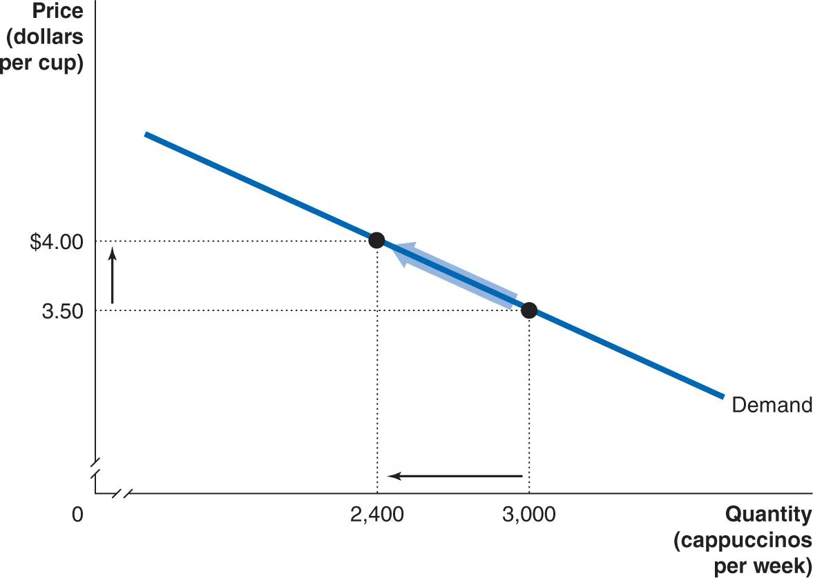
If a Blue Bottle coffeehouse increases the price of its cappuccinos, it will lose some, but not all, of its customers. In this case, raising the price from $3.50 to $4.00 reduces the quantity of cappuccinos consumers demand from 3 ,OOO per week to 2,400. Therefore, unlike a perfect competitor, a Blue Bottle coffeehouse faces a downward-sloping demand curve.

DIAGRAM NARRATION: Real world examples of perfectly competitive markets are not very common. So we will look to the monopolistically competitive market here in this chapter. Recall, examples of a monopolistically competitive firm could be a coffee house, electronic store, or restaurants. Also remember the characteristics of a monopolistically competitive market include many buyers and sellers, low barriers to entry, and differentiated products. This figure shows the downward sloping demand curve for cappuccinos at Blue Bottle. Price is on the vertical axis, quantity on the horizontal axis. And we see the downward-sloping demand curve here due to the law of demand, as we illustrated before. At a price of $3.50, we see Blue Bottle can sell or its quantity demanded is 3,000 cappuccinos per week. If blue bottle decides to increase the price If blue bottle decides to increase the price to $4 per cappuccino, then its quantity demanded will fall to 2,400 cappuccinos per week, illustrating the law of demand. This decrease in quantity demanded is due to an increase in the price for a cappuccino. At higher prices, Blue Bottle will lose some, but not all of its customers, unlike the perfectly competitive firm. Also, unlike the perfectly competitive firm, which faced a horizontal demand curve, as we saw in a previous figure, Blue Bottle faces a downward-sloping demand curve.

Concept Check Question 13.1.1

An increase in the price of cappuccino will increase the quantity of cappuccinos demanded.

A. True.
B. False.

✔ Click here to view answer

Answer: B. An increase in the price of cappuccino will decrease the quantity of cappuccinos demanded.  ✅

Marginal Revenue for a Firm with a Downward-Sloping Demand Curve

For a firm in a perfectly competitive market, the demand curve and the marginal revenue curve are the same (see Chapter 1 2, Section 12.2). A perfectly competitive firm faces a horizontal demand curve and does not have to cut the price to sell a larger quantity. A monopolistically competitive firm, however, must cut the price to sell more, so its marginal revenue curve will slope downward and will be below its demand curve.

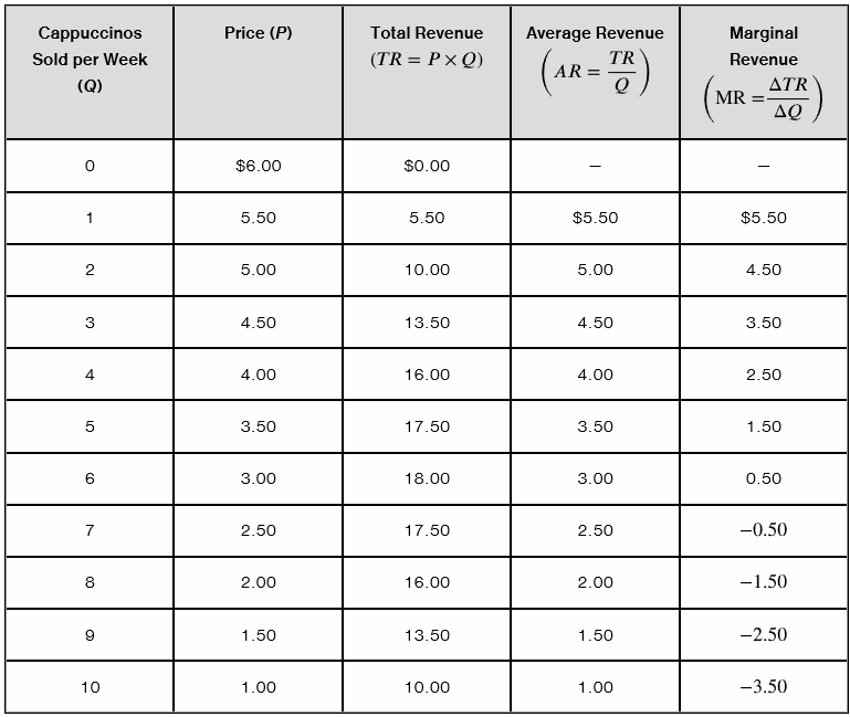
The data in Table 13.1 illustrate this point. To keep the numbers simple, let’s assume that your local Blue Bottle coffeehouse is very small and sells at most 1 0 cappuccinos per week. If this Blue Bottle charges a price of $6.00 or more, all of its potential customers will buy their cappuccinos somewhere else. If it charges $5.50, it will sell 1 cappuccino per week. For each additional $0.50 this Blue Bottle reduces the price, it increases the number of cappuccinos it sells by 1 . The third column in the table shows how the firm’s total revenue changes as it sells more cappuccinos. The fourth column shows the firm’s revenue per unit, or its average revenue. Average revenue is equal to total revenue divided by quantity. Because total revenue equals price multiplied by quantity, dividing by quantity leaves just price. Therefore, average revenue is always equal to price. This result will be true for firms selling in any of the four market structures we described at the beginning of Chapter 12.

Table 13.1
Demand and Marginal Revenue at a Blue Bottle Coffeehouse

Animation: Demand and Marginal Revenue at a Blue Bottle Coffeehouse

A monopolistically competitive firm must cut the price to sell more so its marginal revenue curve will slope downward and is below its demand curve. Demand and marginal revenue at a Blue Bottle Coffeehouse is shown in this table. To keep the numbers simple, let’s assume your local Blue Bottle Coffeehouse is small and sells at most IO cappuccinos per week, as shown in column 1.

If the local Blue Bottle charges a price, from column 2, of $6 or more, all of its potential customers will buy their cappuccinos elsewhere. If it charges $5.50, it will sell one cappuccino per week. For each additional $0.50. this Blue Bottle reduces the price and increases the number of cappuccinos it sells by one.

Third column shows how the firm’s total revenue changes as it sells one more cappuccino. The fourth column shows the firm’s revenue per unit, or its average revenue. Average revenue is equal to total revenue divided by quantity. Because total revenue equals price multiplied by quantity. dividing by quantity just leaves price. Therefore, average revenue is always equal to price.

The last column in this table shows the firm’s marginal revenue. or the change in total revenue as the firm sells one more cappuccino. For a perfectly competitive firm. the additional revenue from selling one more unit equals the price. That will not be true for this Blue Bottle, because to sell another cappuccino, it must reduce the price. When the firm cuts the price by $0.50, one good thing happens, one bad thing happens. The good thing, it sells one more cappuccino, which we call the output effect. The bad thing, it receives $0.50 less for each cappuccino it could have sold at the higher price, which we call the price effect.

The last column in Table 13.1 shows the firm’s marginal revenue, or the change in total revenue as the firm sells 1 more cappuccino. For a perfectly competitive firm, the additional revenue received from selling 1 more unit is just equal to the price. That will not be true for this Blue Bottle coffeehouse because to sell another cappuccino, it has to reduce the price. When the firm cuts the price by $0.50, one good thing happens, and one bad thing happens:

• The good thing: It sells 1 more cappuccino; we can call this the output effect.
• The bad thing: It receives $0.50 less for each cappuccino that it could have sold at the higher price; we can call this the price effect.

Figure 13.2 illustrates what happens when the firm cuts the price from $3.50 to $3.00. Selling the sixth cappuccino adds the $3.00 price to the firm’s revenue; this is the output effect. But this Blue Bottle coffeehouse now receives a price of $3.00, rather than $3.50, on the first 5 cappuccinos sold; this is the price effect. As a result of the price effect, the firm’s revenue on these 5 cappuccinos is $2.50 less than it would have been if the price had remained at $3.50. So, the firm has gained $3.00 in revenue on the sixth cappuccino and lost $2.50 in revenue on the first 5 cappuccinos, for a net change in revenue of $0.50.

Marginal revenue is the change in total revenue from selling 1 more unit. Therefore, the marginal revenue of the sixth cappuccino is $0.50. Notice that the marginal revenue of the sixth cappuccino is far below its price of $3.00. In fact, for each additional cappuccino that this Blue Bottle coffeehouse sells, marginal revenue will be less than price. There is an important general point: Every firm that has the ability to affect the price of the good or service it sells will have a marginal revenue curve that is below its demand curve. Only firms in perfectly competitive markets, which can sell as many units as they want at the market price, have marginal revenue curves that are the same as their demand curves.

Figure 13.2
How a Price Cut Affects a Firm’s Revenue

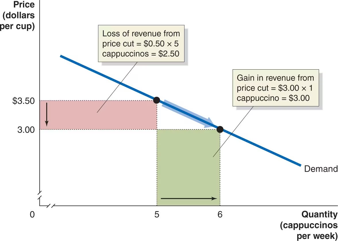
If a local Blue Bottle coffeehouse reduces the price of a cappuccino from $3.50 to $3.00, the number of cappuccinos consumers demand per week will increase from 5 to 6. The coffeehouse’s marginal revenue from selling the sixth cappuccino will be $0.50, which is equal to the $3.00 additional revenue from selling 1 more cappuccino (the area of the green rectangle) minus the $2.50 loss in revenue from selling the first 5 cappuccinos for $0.50 less each (the area of the red rectangle).

Animation: How a Price Cut Affects a Firm’s Revenue

Due to the shape of its demand curve illustrated before. we see in order to sell more cappuccinos, Blue Bottle must lower its price so its total revenue will change. But how much it changes will depend upon the relative change in price versus quantity. So here in this figure, we will illustrate how a price cut affects a firm’s revenue. Price is on the vertical axis, while quantity is on the horizontal axis. The data for this particular graph comes from a previous table.

At a price of $3.50, we see Blue Bottle sells five cappuccinos per week. So its total revenue in this case is $17.50, or $3.50 times five cappuccinos. Now Blue Bottle wishes to increase its sales. So in order to do so, it must lower the price for a cappuccino to $3. As a result. we see it increases its sales by one more cappuccino. Now total revenue due to this lower price is $18, $3 times the six cappuccinos.

Notice Blue Bottle has increased its total revenue by $0.50 by lowering the price of its cappuccinos to $3. Furthermore, we will illustrate this effect by looking at the marginal change for Blue Bottle. Due to this price decrease we see Blue Bottle does increase its sales by one more cappuccino, which is known as the output effect. Now. this is good for Blue Bottle since it is happy to increase its sales. And this extra sale increases revenue by $3.

The one extra cappuccino times the $3 price. However, it does lose $0.50 for each of the previous five cappuccinos, because it must lower the price for all of its customers when it wants to increase sales. This is known as the price effect. So the $0.50 loss times the original five cappuccinos yields a decrease in revenue of $2.50. However, the combined price and output effects increase the marginal revenue by $0.50 when Blue Bottle increases its sales to six cappuccinos due to the lower price.

Figure 13.3 plots the data from Table 13.1 and shows the relationship between the demand curve and the marginal revenue curve for your local Blue Bottle. Notice that after the sixth cappuccino, marginal revenue becomes negative because the additional revenue received from selling 1 more cappuccino is less than the revenue lost from receiving a lower price on the cappuccinos that could have been sold at the original price.

Figure 13.3

The Demand and Marginal Revenue Curves for a Monopolistically Competitive Firm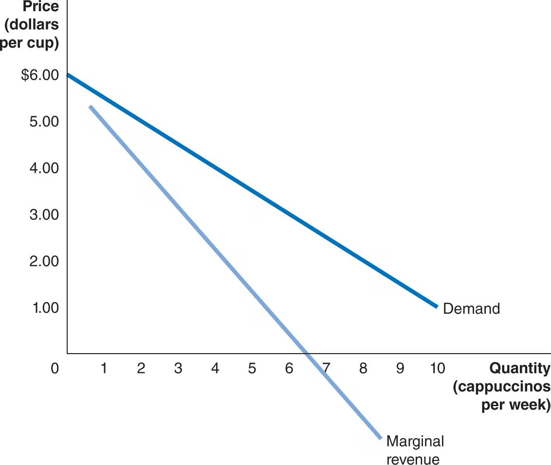

Any firm that has the ability to affect the price of the product it sells will have a marginal revenue curve that is below its demand curve. We plot the data from to create the demand and marginal revenue curves for a Blue Bottle coffeehouse. After the sixth cappuccino, marginal revenue becomes negative because the additional revenue received from selling 1 more cappuccino is less than the revenue lost from receiving a lower price on the cappuccinos that could have been sold at the original price.

Animation: The Demand and Marginal Revenue Curves for a Monopolistically Competitive Firm

INSTRUCTOR: As we saw in a previous figure, when Blue Bottle sold the sixth cappuccino, the marginal revenue it received was $0.50. But the price it charged was $3, which came from its demand curve. In this figure. we will illustrate the demand and marginal revenue curves for a monopolistically competitive firm.

Recall for any firm which can affect price, its marginal revenue curve lies below its demand curve. So here we illustrate the demand curve for Blue Bottle. Recall this data comes from a table in the text. Furthermore, that same data generates a marginal revenue curve below the demand curve.

Recall marginal revenue is simply the change in total revenue divided by the change in quantity. Notice after the sixth cappuccino, marginal revenue becomes negative. That is because of the output effect. The increase in total revenue due to Blue Bottle selling one more cappuccino is less than the decrease in total revenue due to the lower price it must charge for all cappuccinos sold per week. So the marginal revenue curve is always below the demand curve when a firm has the ability to affect price.

Concept Check Question 13.1.2

The monopolistically competitive firm sells______ product and faces ______demand curve.

A. a differentiated; a downward-sloping
B. a homogeneous; a horizontal
C. a homogeneous; a downward-sloping
D. a differentiated; a horizontal

✔ Click here to view answer

Answer: A. a differentiated; a downward-sloping  ✅

If marginal revenue slopes downward, which of the following is true?

A. The firm must increase its price to sell a larger quantity
B. The firm must decrease its price if it wants to continue selling the same quantity.
C. The firm must decrease its price to sell a larger quantity.
D. The firm is unable to adjust price when the quantity sold changes.

✔ Click here to view answer

Answer: C. The firm must decrease its price to sell a larger quantity.  ✅