🙋 Student Q&A (Lecture 3)

Click here to learn about timestamps and my process for answering questions. Section agendas can be found here. Email office hour questions to munger.e1010@gmail.com. PS1Q2=“Question 2 of Problem Set 1”

📅 Questions covered Thursday, Feb 12

🕣 8:18pm
❔ P. 44. Did we start with a demand curve or end up with a demand curve? I don’t understand why we’re doing this.

✔ We only started with the idea that there are two things that determine what you choose:

What you can afford (i.e., your budget) and prices
What you want (i.e., your preferences)

So those are the only things we started with. This is in some ways the important thing that we’re covering. The second thing is to find the demand curve. We didn’t start with a demand curve at all.

🕣 8:22pm
❔ Shouldn’t this be lowercase Q when discussing slide 59.

✔ Good point!

🕣 8:28pm
❔ How do we know which effect is stronger: the income effect or the substitution effect? Do we get it from a diagram? Do we get it from the wording of the word problem?

✔ You’ll typically have to deduce which effect is stronger based on some sort of information that he gives you in the problem. In different problems, he will give you different information. Sometimes the information that he gives you that allows you to detect whether the income or substitution effect is stronger is a diagram. Other times, it is the wording of the problem. So, either of them will work. It could possibly be other things. Maybe they’ll have a table which lists how much you buy at different prices. Any of those will work. The key thing is you understand the system and then you can work through it. We’ll do some examples as we go through.

The bottom line is this: In some questions, there’ll be some information that tells you what actually happens to demand as the price changes. Demand is just another name for the combined effect. Rather, the combined effect is another name for demand. So if demand goes up, the combined effect is positive. If demand quantity demanded of the good goes down, then the combined effect is negative. You can be told that demand goes up or that quantity demanded goes up or the quantity demanded goes down from a table, from a sentence, or from a diagram. They’re all the same, and you just have to have this fact at your fingertips. You have to understand that combined effect just means how much you buy.

So there’s lots of ways he can tell you that the person bought less after the price change. No matter how he tells you that, you need to understand because you have all the facts at your fingertips that if they bought less, the combined effect is negative. That will allow you to do things later on in the problem about whether the IE or SE is stronger given what you know about whether the IE and SE are positive. We’ll talk about that later on.

🕣 8:31pm
❔ IE and SE. Make it systematic.

✔ There will always be a significant amount to remember, but I can give you a framework.

🕣 9:45ish
❔ 1. o make sure I’m understanding this properly, on slide 8, if we say that maybe Keira started at point D, the non-optimal point, in order to get to the optimal point C, she consumes less of the good that gives fewer utils per dollar at point D and more of the good that gives more utils per dollar at point D. Is that correct?

To extrapolate from here, if there is a combination of goods that we find is non-optimal based on marginal utility per dollar spent, will it always be true that consuming less of the good that gives fewer utils per dollar and more of the good that gives more utils per dollar will get us to the optimal point?

✔ video

🕣
❔ Giffen good: why do they go up?

✔ covered in video

🕣
❔ 1. (This we can do on Sunday/next section if you prefer) I love the charts that Bruce did for SE and IE—slide 39 for price going down for normal goods and slide 61/62 for price going down for an inferior good. Can we work through the same logic and charts for normal and inferior goods when prices rise?

✔

🕣 9:51pm
❔ Can we get extra exercise questions on combined effect? I am still not sure I got it 100%.

✔ Inferior good Price rises. What happens?

SE? ↓ IE: PP↓ IE↑ (The price of the good rises, so you have less money at the end of the week. You feel poorer and your purchasing power has decreasedd. Therefore you wil be forced to buy more of inferior goods, including the inferior good in question. As a result, the income effect will be positive.) CE: Ambiguous. If SE>IE: ↓ If SE<IE: ↑ ← Giffen good because the price rose and you purchased more.

In many economics classes, they will refer to what’s known as the law of demand. The law of demand is what most marketers and businesspeople think of, which is that if you lower your prices, people will buy more of the good. This is separate from the idea of a Veblen Good, which I think is also legitimate and which I think businesspeople also do take into account and should. But in general, they’ll also be thinking of the law of demand, which is that when you increase your prices, people will buy less, and if you decrease your prices, people will buy more. This contradicts the law of demand and is therefore a Giffen Good because price went up and people bought more.

Normal good and prices Rise:

SE: ↓ IE: PP↓ It’s a normal good, so when you are poorer, you buy less. Therefore IE↓ The two arrows go in the same direction, so you don’t have to think about which one is stronger. Therefore, the combined effect is that you purchase less of the good.

Inferior good will only have a price going down SE: ↑ IE PP↑ This is inferior, so when yo uhave more money you avoid it like spam. IE↓ a If SE↑ > IE↓, then CE↑ b If SE↑ < IE↓, then IE↓ On line b, The price went down and you purchased less. That’s contrary to the law of demand that says when the price goes down, you buy more, therefore, it’s giffen. In general, with an inferior good, if the price of the inferior good changes, then if the income effect is stronger, it will be a Giffen good, as exemplified by the web page that we covered earlier with those diagrams on it. You will have a Giffen good when you have an inferior good and the income effect outweighs the substitution effect.

🕣
❔

✔

📅 No Section on Sunday, Feb 15

No Section today. Please email any questions.

📅 Questions covered Thursday, Feb 19

🕣 8:18pm
❔ Did you mention something called Vaeblen Goods? Is that fair game for a graduate paper?

✔ Yes

🕣 8:18pm
❔ Can I ask why the CO is higher up in the graph making calls to france negative? Instead of directly shifted over??

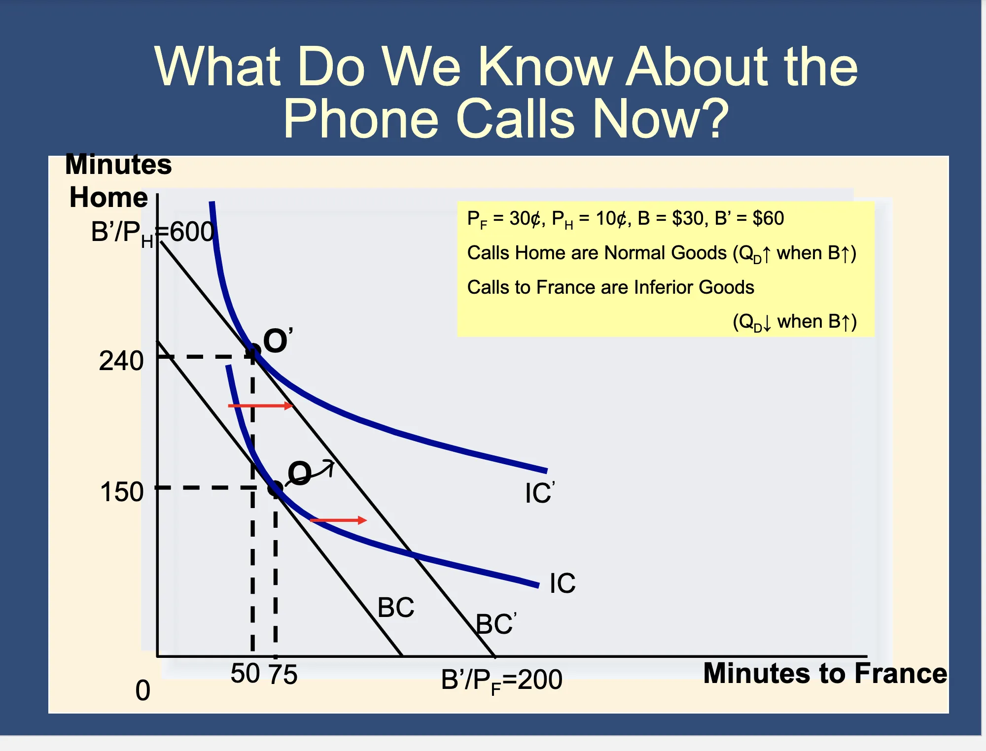
✔ It’s like this because people are complex, and they may react differently when their income goes up. I guess in this situation, this is a situation that we understand well, so why don’t I put it out to you folks? What’s going on in this diagram specifically related to minutes to France?

Exactly, Safira. It’s an inferior good.

What we know about this is that someone in the chat room said that the motto of microeconomics is like this because people are complex. Yes. At least the one thing that we can rely on is that they have objectives and they try to pursue those objectives. That’s the only simplifying factor we get.

In this situation, we know that it’s an inferior good. One thing you need to know, and this is covered in other slides, is that when the budget constraint shifts outward like this, it means that your income has risen. The budget has risen, so you have more money. This is clearly illustrating what happens when you have more money. If you want me to go over that, we can absolutely go over that. There’s a whole presentation I can do.

We did that in the previous lecture; we covered that, but sometimes it requires a little bit of repetition. Anyway, we know that in this situation we are wealthier because the budget constraints shifted outward. We can see from the diagram that, at the new optimum o prime, we are indeed consuming more minutes home and fewer minutes to France. We’re consuming fewer minutes to France when our income rose. Minutes to France must be an inferior good.

🕣 8:21pm
❔ Slide 19 the CO moves parallel but slide 20 CO shifts up?

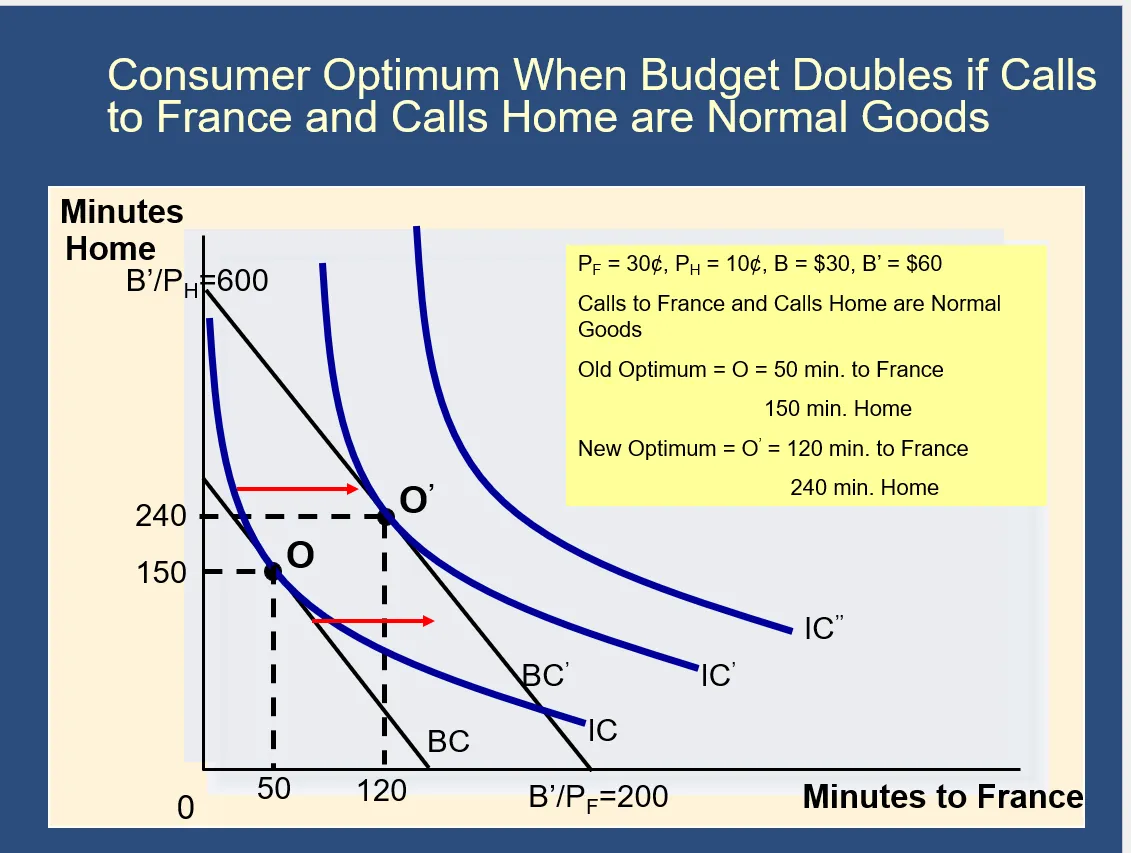
✔ Here, both goods are normal, so when your income increases, you consume more of both goods. Really glad we had a chance to review that.

🕣 8:45pm
❔ Question. This is a practice problem on Pearson. If a consumer is willing to give up 3 units of good X for 1 additional unit of good Y, what is the marginal rate of substitution of X for Y? The answer is 3. I had it at 1/3 which was wrong.

✔ The marginal rate of substitution, by definition, is the amount of a good Y that you’re willing to give up to get one unit of good X.

There is a difference between the marginal rate of substitution of x for y and the marginal rate of substitution of y for x. It’s always the number of units of the second thing that you’re willing to give up to get one unit of the first thing.

That’s the definition. We need to know how many units of the second thing you’re willing to give up to get one unit of the first thing. In other words, we need to know how many units of Y you’re willing to give up to get one unit of X. This, by the way, corresponds to how we usually lay it out on the axes, so nothing is different here.

Bottom line: How many units of good y do we give up to get one unit of good x?

We know that we are willing to give up three units of x to get one unit of good Y, but that’s the opposite of what we need. If we are willing to give up three units of good x to get one additional unit of good Y, it must mean that the marginal utility of good Y is roughly three times the utility of good x. We must simply like good Y three times as much if we’re willing to give up three units of good X in order to get one unit of good Y. Therefore, it stands to reason that we would be willing to give up only a third of a unit of good Y to get one unit of good X, because after all, we like good Y more than we like good X.

This is the answer that you’re looking for. We are willing to give up one third of a unit of good Y in order to get one unit of good X. Therefore, the marginal rate of substitution of X for Y is one third.

MRS = MUx/MUy We’re told: A consumer is willing to give up 3 units of good X for 1 additional unit of good Y If that’s true, it must be that the additional happiness you get from good Y is three times the additional happiness you get from good X. In other words, MUy = 3 × MUx. Therefore, MRS = MUx/MUy = MUx/(3 × MUx) = 1/3

MUh = 3 × MUs

You would give up 3 sandwiches to get one hamburger. How many hamburgers would you give up to get one sandwich? Well, since you like hamburgers three times as much, you’d only give up a third of a hamburger to get a sandwich.

🕣 9:03pm
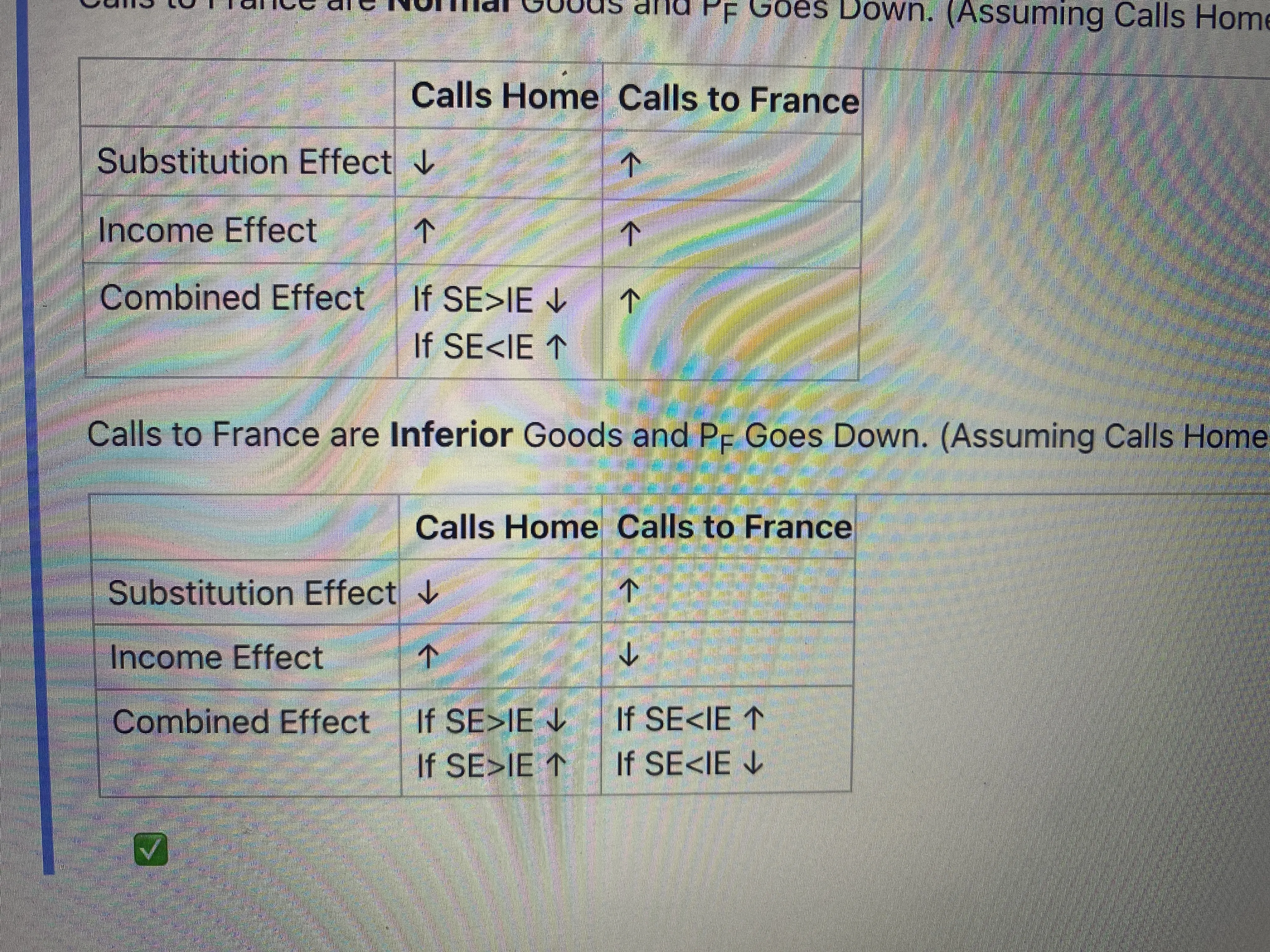
❔ I’m catching up on Thursday’s section and have a question about the SE and IE on the Pf of Inferior Goods chart, where the price of the inferior good goes down. Since both the normal good and inferior good have these opposite arrows for SE and IE, can we infer anything about one by knowing the combined effect of the other? For example, it seems to me that if the IE of the inferior good is larger, so that the amount of calls to France (for example) goes down, then the SE for the calls home can’t be the larger effect because then the amount of each would go down even though you’re effectively richer. So, in that case, I would extrapolate that if the IE is larger for the inferior good, it must also be larger for the normal good, right? Do those effects go hand in hand for both goods? Or are there times when the effect of one would be larger for the inferior good and the effect of the other would be larger for the normal good?

✔ It’s important to note that in an analysis with only two goods, you can’t have both goods being inferior. This is because if you get more money, you’re going to have to spend it on something. You’re still going to want to spend all your money, and if both goods were inferior, you’d want to buy less of both, and you’re richer. Why are you buying less of both goods? It wouldn’t make sense in a situation where goods are considered to be good.

We’re always going to have one good be normal, and I suspect that with a normal good, the arrows will go in the same direction, but let’s check, because we’re looking at the good whose price isn’t changing, and that may be different.

Another thing to bear in mind is that we aren’t going to be too concerned about this particular situation, because mostly what he’s interested in motivating and exploring is Giffen Goods. Giffen Goods looks at the combined effect of the price of the good whose price changed, not the other good. Now we’re looking at the other good, so again I might just call time on this.

🕣
❔ typo? ✔ Just checked, and they look good to me.

🕣 9:13pm
❔ Is it helpful to review your website? Also you mentioned reading the chapter? I can’t seem to open it in pearson? Is it because I bought the cheapest version?

✔ Yes, I think it’s hugely helpful to review the website. The slides are the foundation of the course, so I think they’re your priority. The website is meant to supplement Bruce’s lecture and the slides. First, you want to use the slides, and then you can return to mine. Occasionally, some students will prefer to use the slides or my website or the sections first, but I think that’s rare, and that’s not how they’re designed. They’re designed to complement the core from the slides and the lecture.

Reading the chapter can be helpful. It can familiarize you with different ways of stating things, different vocabulary for the same thing, which can be helpful on the exam, but it can also get you off on side tracks. To illustrate that, I’m actually going to go to the next question that someone put in the chat room.

The following question illustrates something that you’ll see in the textbook, which you absolutely aren’t responsible for. While I do think that it can be helpful to review the textbook, the textbook will contain things that you’re not responsible for, and it can be very, very hard to work through those things.

It’s important that you first study the slides in the lecture so you can have a good sense of radar to think quickly. I don’t remember anything like this from the slides, so it’s like you do the reading last. In the early on, I suggested that if people want, they can get the Hubbard and O’Brien book, whereas there are going to be some things in Pendyke and Rubenfeld that we don’t cover, such as this. We will do heavy coverage of the material in Hubbard and O’Brien, and that will, in general, be at a lower level than we do here, which is great. That means it’s easier. I know when I’m learning hard material, it’s much easier.

I’ll go into ChatGPT and I’ll be like, “Make this simple,” and then I can read the hard version, but first I need to explain it to me like I’m five. The Hubbard and O’Brien will be the easier one that you can start with.

🕣 9:14pm
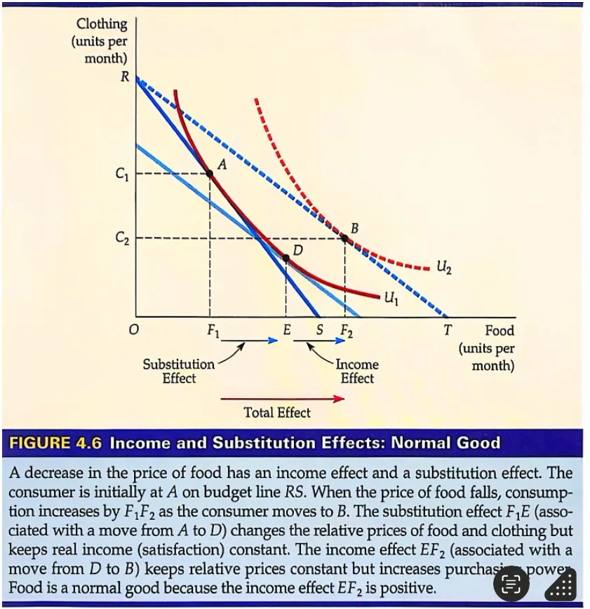
❔ Would you mind walking me through this chart? ✔ Only if you stay late. 😂

🕣 9:18pm
❔ Does the substitution effect still apply if a good’s own price is changing?

✔ Yes. The substitution effect occurs when the price of the current good changes or when the price of a different good changes.

It doesn’t have to be the price of the other good that changes for the substitution effect to apply. The substitution effect can also apply to a good when its own price changes.

Total utility on graph

🕣 9:19pm
❔ How does TU increase or Decrease look like as a change in the graph with two normal goods with IC and BC?

✔ Total utility is indicated by your indifference curve. If you get on a higher indifference curve, then your total utility has increased. The definition of indifference curves is that they tell you what your level of utility is. We therefore know that if you move on to a higher indifference curve, you are happier. That’s what our mission is: to always get on a higher indifference curve.

Let me know either on mute or in the chat room if you have any follow-up questions.

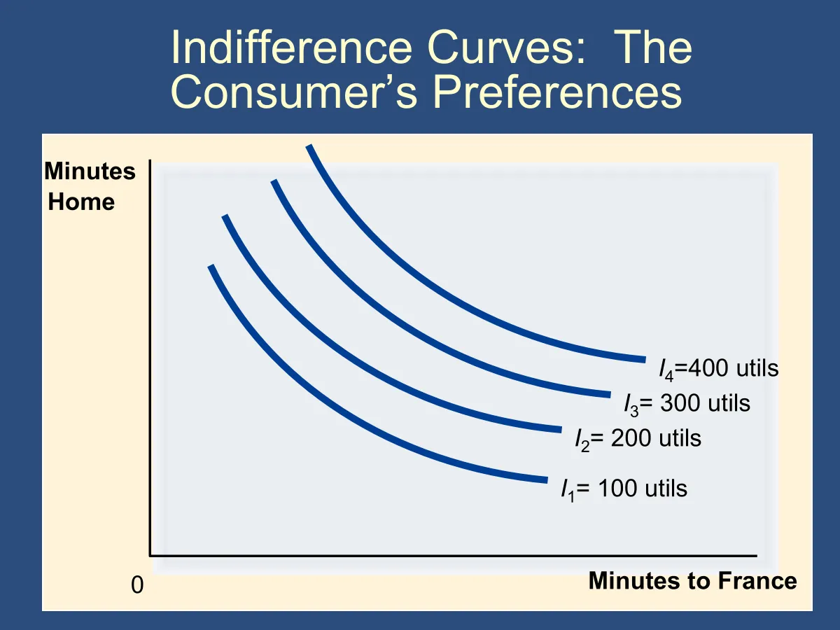
BC movement when income increases

🕣 9:21pm
❔ Check class slides but how does the BC move if income increases but price of goods remain the same

✔We discussed this earlier, but it shifts to the right so that you can purchase more goods. This illustrates nicely how there’s only so many questions that can be asked here, and so the more you study, the more you kind of fill in the gaps.

Where CO moves when BC changes

🕣 9:21pm
❔ How do you know where the CO moves to when the budget constraint changes

✔ Wherever the budget constraint is, there will always be exactly one point where an indifference curve is tangent to the budget constraint. Therefore, to find the new consumer optimum, you just find the new point where there is an indifference curve that is tangent to the new budget constraint. We can see this in the slides, like the slides above.

Steepness of BC slope

🕣 9:23pm
❔ What does the steepness of the slope of the BC mean and what does it mean when it is more flat

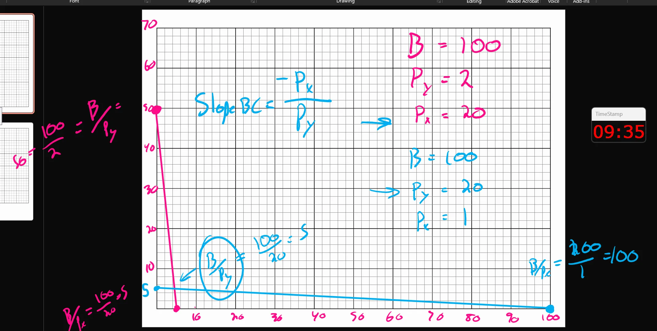
✔ We actually have a very good answer to this using our formulas, so this is how we draw connections. We have a formula that says: Slope of BC = -Px/Py.

When the slope of the BC is flat it means that p_x over p_y is small. That means that Px is small compared to Py.

Bottom line: Px is small compared to Py when the curve is more flat.

As always with the budget constraint, you can understand the shape or the steepness or flatness of the budget constraint by looking at the two endpoints. We know that for the two endpoints, they are determined by b/px and b/py.

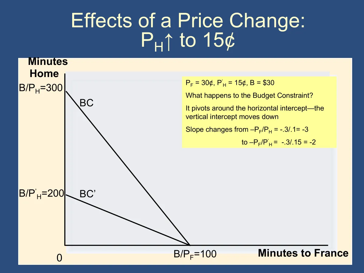
In the flat budget constraint, you have a higher price for good Y so that good Y is high compared to good X. Therefore, px is small compared to py.

🙋Can we get a real-world example of the steepness of the slope of the budget constraint?

Determining combined effect

🕣 9:27pm
❔ What is the best way to determine the combined effect? Slide 40 lecture 3? (consider going back to section recording)

✔ So the green line diagram, the thing that we’re skipping and you’re not responsible for, is a way of breaking down the actual behavior that people do into an income effect and a substitution effect. The combined effect is just what you get when you combine those things back into one. The combined effect is just what people actually do. That’s what the combined effect is: their behavior.

If you want to know what the combined effect is, just look at the question and ask: what in the question tells me what people are actually doing? If a demand curve is sloping down and a price just rose, if you look at the curve, it says that people are buying less stuff. Consumption went down. That’s what people actually did. The combined effect is a decrease. If they just tell you that the person buys less, then you know that the combined effect is a decrease.

All you have to do is just read the question carefully and keep your head on, and you’re good to go.

SE, IE, CE direction for normal goods

🕣 9:35pm
❔ L3 Slide 54 would you say if the goods are normal, the SE and IE are going up or down or just the same the CE is the same direction as well? Explain in an example?

✔If the goods are normal, then when you look at the IE, SE and CE for the good whose price changed, all three of the arrows will go in the same direction.

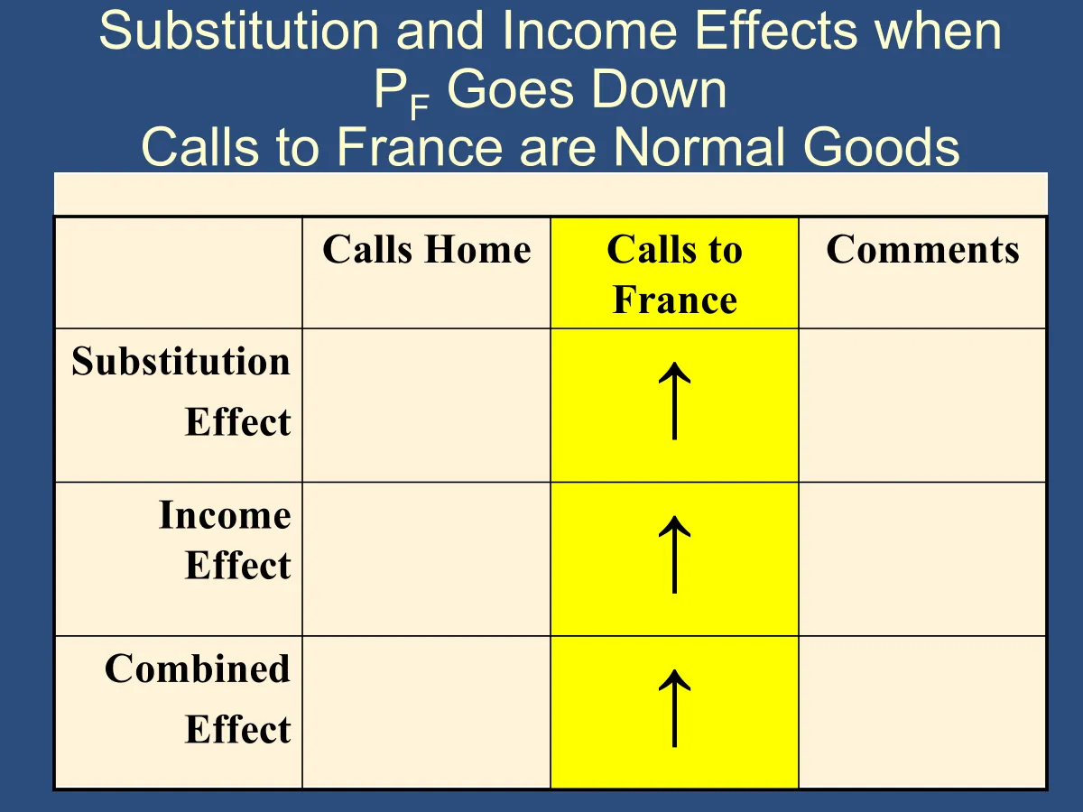
This is what happens most of the time. This is what happens when the price changes on a normal good. Normal goods are normal, so when the price of any good goes down, we think, “Ah! That book, that item feels relatively less expensive. I should probably buy more of it because it’s a better deal.” That’s the substitution effect, and the income effect says, “Ah! It’s a normal good, so its price just went down. I’m feeling a little bit richer. I don’t have to pay as much for it, so I’ll buy more.” If I feel I got two reasons to buy more, then I’ll definitely buy more, so that’s the combined effect.

You just kind of combine all three of them, and all three of the arrows go in the same direction. It all lines up simply, and you don’t have to think about which effect is stronger. If the price increases, then once again all the arrows will line up; they’re just going to go in the opposite direction.

France SE up on Slide 54

🕣 9:38pm
❔ Slide 54 L3 why does it say France for SE up when above the caption states the Price goes up or is that just the effect because in relation to the price change (am I reading the chart correctly?)

✔I don’t know what version of the slide you’re looking at, but I can say that in the version of the slide that I have, the price of a call to France goes down. Because the price goes down, the substitution effect means you’re going to buy more.

Inferior good on Slide 62

🕣 9:39pm
❔ Hard time interpreting Slide 62 L3 in regards inferior good

✔This is a classic question, so this is definitely something you want to be comfortable with. This is key to explaining the story about how Giffen goods work, so let’s go through all three steps.

We’ll do the substitution effect. Clearly, the price went down, so it’s very natural when something gets cheaper that you’re going to substitute and buy more of it. I like to think of the substitution effect as the “Deal Hunters effect.” If you go through the process, when the price of a call to France goes down, relative to other goods it now looks cheaper, so you’ll buy more of it. I’m going to trust that you get that, so let’s move on to the income effect.
For the income effect, as I’m describing the process that I encourage people to follow, if you want a written-out process, step one is to ask: “Are you feeling richer or poorer?” You need to have an answer to that based on the price going down. Well, if a price goes down, I have to spend less on that good, so I feel richer. My purchasing power has risen, and therefore I feel richer, and when I feel richer I buy fewer inferior goods. That’s the clincher. Because a price fell, I feel a little bit richer; I don’t have to spend as much on that good, so I can avoid the inferior goods. I’m going to buy fewer calls to France, so that’s why that arrow goes down.
I think for the third one, we’ve already done a couple examples of if IE is bigger and the income effect goes down, then the combined effect will go down. If SE is bigger and SE is going up, then the combined effect will go up because SE will win.

IE direction for inferior good, Slide 61

🕣
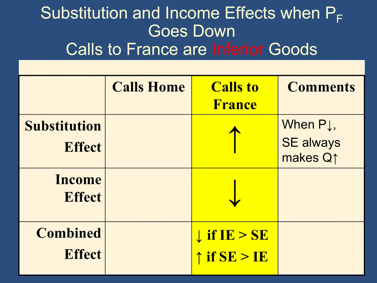
❔ Slide 61 why would the income effect for France go down if the price goes down and it is an inferior good? (Are we only focused on FRANCE and not HOME when reading this chart) ✔Yes, exactly. On this slide, we’re only looking at the substitution income and combined effects on France because we’re in the yellow middle column. We’re only looking at that being caused by the change in the price of a call to France.

For the income effect, in particular, the way that it goes is: a price went down; therefore you have to spend less money; therefore you’re feeling a little bit richer; therefore, whenever you feel richer, you buy fewer inferior goods, so you’re going to buy fewer calls to France.

Separating SE and IE for inferior goods

🕣 10:11pm
❔ Slide 62 how do you talk about SE in regards to an inferior good when you are also discussing IE how to separate the two?

✔The nice thing about IE and SE is that we do have the recipes, and you want to understand the recipes deeply so that they really make sense. That’s the first step.

The second step is that now that you understand them and they totally make sense, you’re going to forget them. You need to practice them until you can do them independently without any prompting. You just practice a lot until you kind of memorize them.

You - if we aren’t given any other information other than what’s on the table, you don’t know which is stronger. The only thing you can write down is a conditional: if I is greater than SE, then this; if SE is greater than IE, then this. That’s literally all you know, and it’s all you can write down and it’s all you can ask.

However, sometimes he gives you additional information, and you have to pay attention to any clues that he has given you. For example, suppose somewhere in the problem set you are told that when this happens, the person calls France less. In that situation, you’ve literally been told that the person calls France less; therefore, you know that the combined effect must be a decrease. Therefore, you can deduce that the income effect is stronger than the substitution effect.

As an alternative, he could also tell you that calls to France are a Giffen good. Now you know, and this is where some of the questions can be hard, because you have to pull in different pieces of information and why they all have to be at your fingertips.

You know that, for a Giffen good, when a price goes down you buy less of it. Since the price went down, we know that you’re going to buy less of it. In this situation, you have to observe that he told you that it’s a Giffen good and know that that’s relevant. You have to therefore conclude that they’re going to buy fewer minutes to France, and therefore you know that the combined effect is down. You can conclude that IE is greater than SE.

Another thing that he could say is that calls to France have a downward sloping demand curve. We know that if you have a Giffen good, it’s an upward sloping demand curve. We know it’s not a Giffen good, so we know that things are going to be the opposite of the last example. If you visualize a downward sloping demand curve, when the price declines, the quantity demanded increases. Given that the price of a call to France did decline, we know that the quantity demanded of a call to France must increase. Therefore, the combined effect must be a positive.

If he tells you anywhere in the problem that France has a downward sloping demand curve, you can conclude that the combined effect of a price drop is you’re going to buy more calls to France. Therefore, you can conclude that SE must be greater than 90. You could reason that out. That’s considered fair game, but I don’t think that most of this, again, this would be the hardest question on the exam. I think most people can be like, “I don’t have to get the hardest question on the exam,” but we still train for it. If nothing else, to know that okay, that’s what the hardest question in the exam looks like.

Dana spending entire budget

🕣
❔ In rob’s website notes how do we know Dana is spending her entire budget?

✔ We’re told:

📅 Questions covered Sunday, Feb 22

🕣 7:42pm
❔ You recommend another economics book. Could you remind me which one it is?

✔ In e1000 Essentials of Economics, we use Hubbard and O’Brien, and I think it heavily influences his approach to teaching, or I think it aligns better with his approach to teaching, and so that can be a useful resource.

If you have Hubbard and O’Brien, you can email me and say, “Hey, what chapters correspond to this lecture?” and I’ll be happy to let you know. You only need the Hubbard and O’Brien that has economics, microeconomics, and macroeconomics. Economics can be divided into microeconomics and macroeconomics. Obviously we’re doing microeconomics; it’s in the title of the course. The Hubbard and O’Brien economics, so the microeconomics book is the one that you want.

Microeconomics 3rd Edition

by R. Glenn Hubbard (Author), Anthony Patrick O’Brien (Author)

🕣 7:45pm
❔ If the price of a normal good rises what would be the best way to explain what happens to both SE and IE how would you state they impact each other…?

✔ See video

🕣 7:56pm
❔ On slide 21, it seems that O’ is not on the budget constraint curve.

The Min Home = -3 Min Fran + 600. if we look at optimal point O’ (50,240), when min to F is 50, the min home should be -3*50+600 = 450 instead of 240.

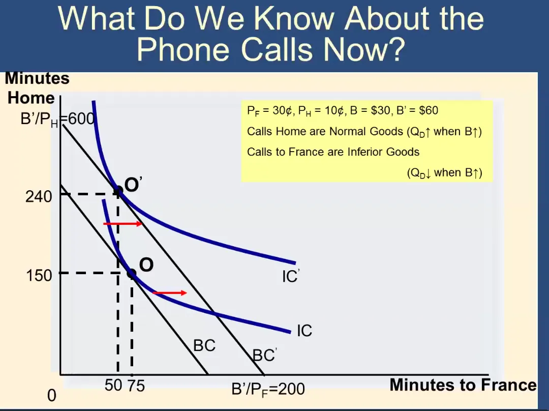
✔ You’re right! O’ is not on the budget constraint!

Are you spending your money? 240*.1 + 50*.3 = 24+15 = 39

You are right that the numbers aren’t working here. I can let Bruce know.

What you need to get from the diagram is that if the budget increases and the quantity demanded of minutes to France decreases then the good is an inferior good.

🕣
❔ Also in slide 23, The Min Home = -3 Min Fran + 600. if we look at optimal point O’ (120,150), when min to F is 120, the min home should be -3*120+600 = 240 instead of 150.

However, if O’ sits on (120, 240) it has the same vertical position as point O(50, 240), which does not make sense to me because if budget goes up and Min Home is inferior good, the consumer will buy less instead of buying the same.

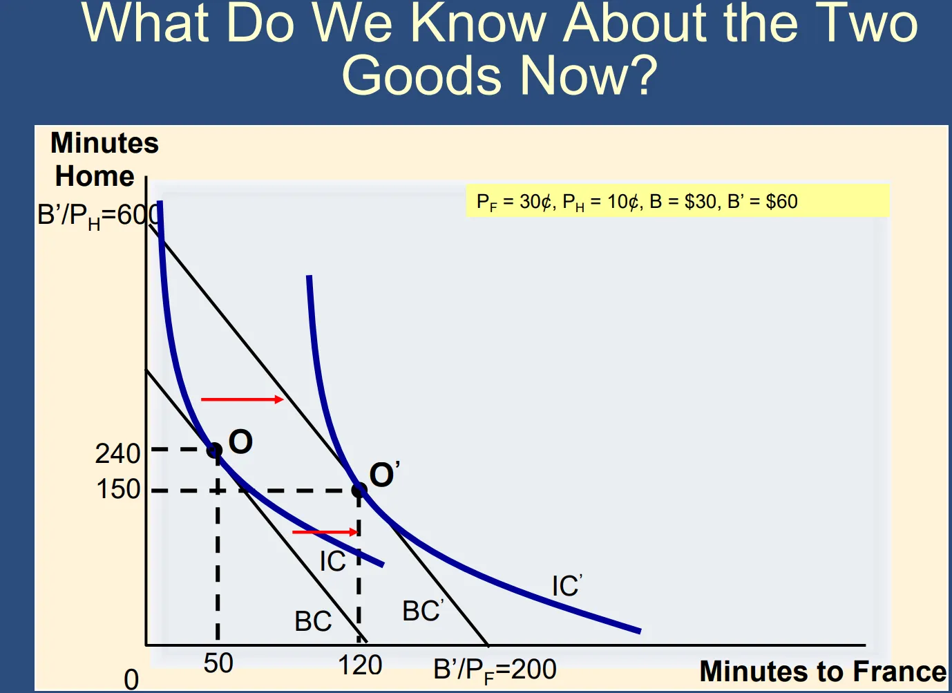
Given Min Home is inferior good, I believe point O’ here on slide 23 should locate somewhere that Min to Fran is larger than 120.

Please let me know if I was wrong.

✔ 240*.1 + 50*.3 = 24+14 = 39 So you spend 39 at O and you spend

120*.3 + 150*.1 = 36+15 = 51 So his diagrams would be corrected if he just updates the budget numbers on them. Terrific observation!

🕣 7:54pm
❔ Could I ask you to clarify some terminology.

On the IC, when we say steeper, we are talking about the upper area of the curve where dY it a bigger number than when X is 1 correct?

When we say flatter, we are talking about the lower area where dY can be less than 1 when compared to X is 1?

So when we say the curve is flattening, we are saying the dY is reducing as it goes down the curve so the consumer is willing to give up less Y for 1 more X as we go down the curve. Is this logic and wording correct?

✔ Steeper just means that something is pointing more downward and flatter just means that something is flatter - pointing more horizontally. Indifference curves typically have what we call a convex shape. As you mention, in the upper area they’re steeper, more up and down, whereas in the lower part, farther off to the right, they are flatter, more horizontal. I think that’s what you’re getting at there, and if that’s what you’re saying, absolutely right.

We could talk about budget constraints also being steeper and flatter, but for indifference curves they tend to have this shape. Now, indifference curves can have other shapes. We’re focusing on the shape that we see most common, which is that concave shape. That’s the one where, at the high points, it is steep, meaning more up and down, and at the low points it is more flatter.

🕣 8:04 pm
❔ I understand that when the price of a normal good rises the SE and IE go down. But do they offset each other or impact each other in anyway or can we just say you buy less of the normal good? ✔ Price rises → good is relatively more expensive → SE↓ Price rises → you are poorer (lower PP) → buy less of normal goods → IE↓ To answer your question, which is a great question, they don’t really interact or impact each other in any way. They’re just like separate things.

You analyze the substitution effect with one pattern.
You analyze the income effect with the other pattern.

You don’t have to know about the income effect when you’re doing the substitution effect, and you have to know about the substitution effect when you’re doing the income effect, so they’re just really separate. Great question.

🕣 9:07pm
❔ Can I ask why we would rearrange this formula and when we would need to do this? I understand the CO and the formula itself.

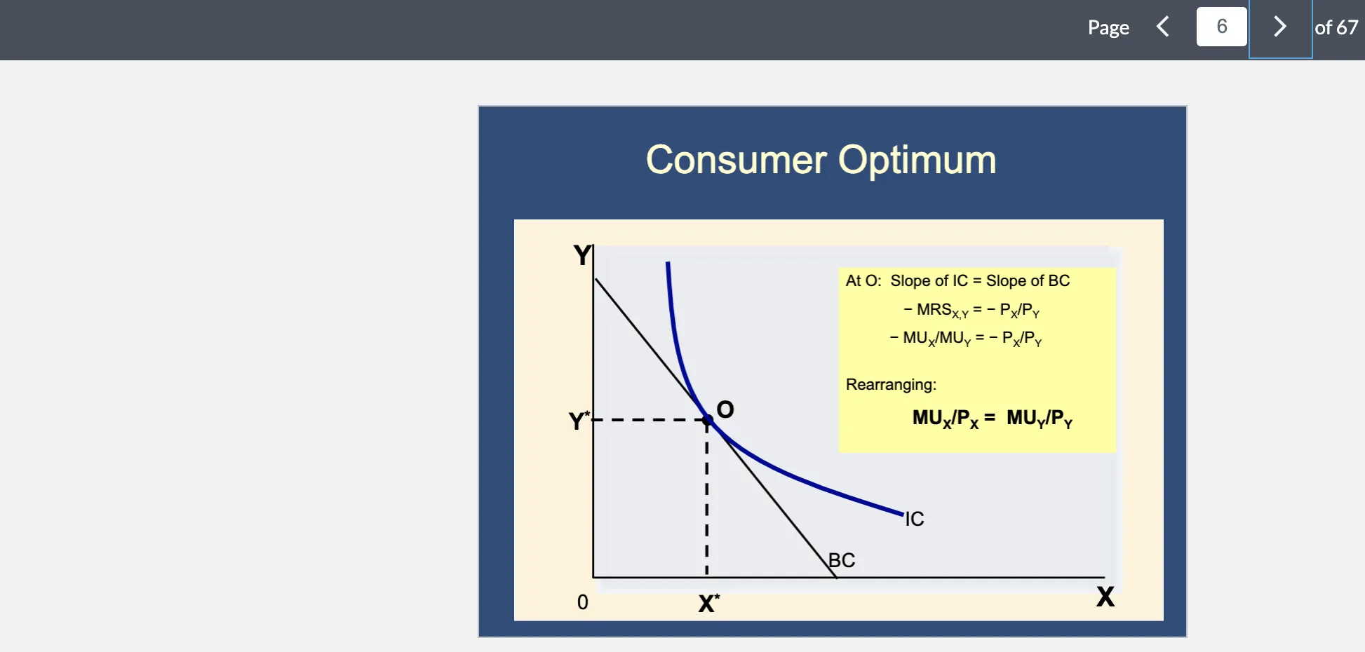
✔ This is what is called in math a proof. You start with some things that you know and then derive or figure out other things that you also know. When we say you know these, you know them with mathematical certainty.

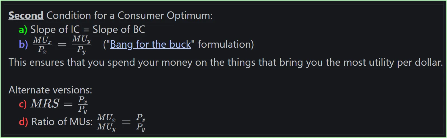
At the top of this slide, we have convinced ourselves that, when you’re optimizing, the slope of the IC equals the slope of the BC. We use that to figure out another fact, and we use the second fact to figure out a third fact. We figure out the third fact to figure out the fourth fact. All four facts are useful for us when solving problems.

The reason that we’re rearranging these things and substituting in is because it helps us with facts that allow us to draw conclusions. The one that we’re most interested in is the last line. We’re most interested in that fact, but this slide is basically the four different versions of the second optimization condition.

🙋‍♀️ Can we put numbers on this? We’ll use this example: https://1010.robmunger.com/l3/isdanaoptimizing/

✏️ At her present levels of consumption of goods X and Y, Dana is spending her entire budget, and her
MRS X,Y = 5, PX = $9**, and **PY =$ 2.
Is Dana consuming the optimal amount of goods X and Y?

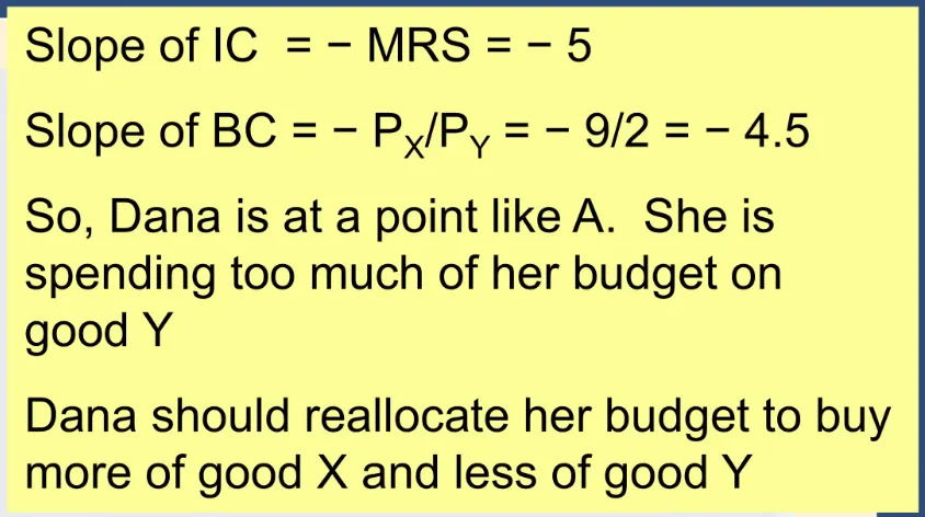
We are told that the MRS for Dana is 5. We know that the slope of the IC = -MRS. Therefore, for Dana, at her current consumption, Slope of IC = -5. We also want to think about the slope of the BC. Slope of BC = -Px/Py Slope of BC = -9/2 = -4.5 Because Slope of IC ≠ Slope of BC, Dana isn’t optimizing.

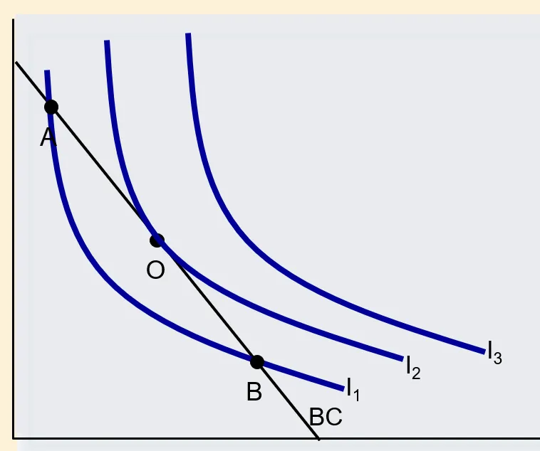
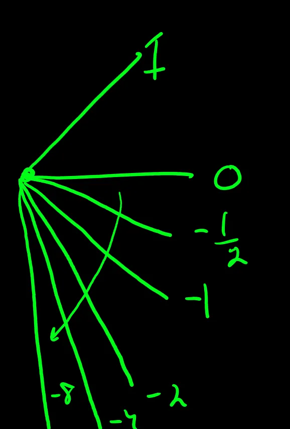
Let’s put this on her diagram. She’s spending all of her money, so she is on the BC. Is she at the tangency point, below it, or above it? At O, A, or B? At O, the steepness of the blue curve and the black curve are the same, but we know that for Dana the steepness of these two curves isn’t the same. In fact, we know that the steepness of the blue curve, which is the IC, is -5, and the steepness of the black curve, which is the BC, is -4.5. Because -5 is a more extreme number than -4.5, we know that the indifference curve is steeper than the budget constraint, and that allows us to answer this: At which point are we at? Are we point A or are we at point E? Which one has a steeper indifference curve than the budget constraint?

Steeper = more negative. -3 flatter -4.5 medium -5 steeper 0 is flatter.

Steeper → the slope is far from zero. Flatter → the slope is closer to zero.

The reason why this is true is that slope is Δy/Δx, and Δy tells you how much you are going up and/or down.

🕣 8:31pm
❔ If we have two goods, and one has more marginal utility per dollar than the other. In order to get to the optimum, we should decrease the consumption of that good until it becomes equal to the Mu/p$ of the other good (Mux/Px = Muy/Py).

But isn’t this counter intuitive? Why would I decrease the consumption of something that is giving me MORE MU per dollar spent? Is this only because of the budget constraint? Suppose budget is not mentioned at all, should we choose the good that has more Mu per dollar?

Sorry I think I got the math wrong. If Mux/Px is higher, in order to make it lower we need to reduce the numerator (Mux) not the quantity consumed and that can be done by increasing the consumption not decreasing it. If you could still discuss this in the next section it would be very helpful!

✔ You should always consume more of the good that has higher utils per dollar. That’s it, that’s all you need to know.

When you consume more of the good that has more utils per dollar, you get a little sick of that good. Because of decreasing marginal utility, the marginal utility per dollar of that good will decline because you’re sick of it. It will keep on declining until it’s equal to the marginal utility of the other good. When they’re finally equal, you’ve satisfied the second optimization condition and you’re done.

In your second explanation, you nailed it. If the marginal utility per dollar is higher to make it equal the other one, we need to make the marginal utility per dollar lower by consuming more of the good. Again, we consume more of the good, which makes the marginal utility per dollar lower until the two are equal.

MUco /Pco = MUch / Pch

🕣 8:37pm
❔ When approaching a problem, we can typically decide which good to put in the x or y axis, unless the question indicates which good goes in which axis? Would choosing a different axis affect our results regarding MRS & consumer optimum?

✔ In all of the problems that I can think of, it won’t matter which good you put on which axis.

🕣 8:38pm
❔ 1. I am a little old school and take notes by hand. Would I be able to use these for the exam? Do you recommend I use a word document instead?

✔ You’re more than welcome to use any sort of paper notes that you want on the exam. You’re also welcome to use a Word Doc. Really, it’s whatever you prefer. If you like, it may be easier to search through a Word Doc, so there are advantages of doing a Word Doc, but you could transition it. That’s your call. I don’t know.

🕣
❔ When calculating the MRS along an IC, if the result is a decimal, it indicates it will be further down along the curve? See screenshot below: ✔ That’s a good intuition.

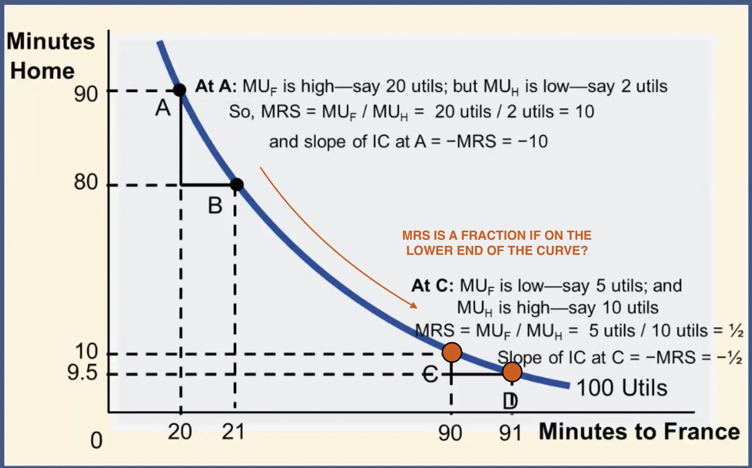
I’m saying that it’s an intuition because I think we could say it a little bit more precisely, so let me try to say it more precisely.

Most indifference curves will have a standard convex shape. They have that beautiful curve that you highlighted in your diagram. They get flatter as you go down. If you have a curve like this, then MRS will get lower as you slide down the curve. Eventually, we expect it’s going to get low enough so it’s a fraction or a decimal, and that’s going to happen lower on the curve. Once it gets low, it’s just going to keep getting lower and lower and lower and closer and closer to 0.

Now we get to go back to what Claire said earlier. The slope gets flatter and flatter and flatter, which means closer and closer to 0. I could do this in terms of slope; I’m just going to do it in terms of MRS on the diagram.

🕣
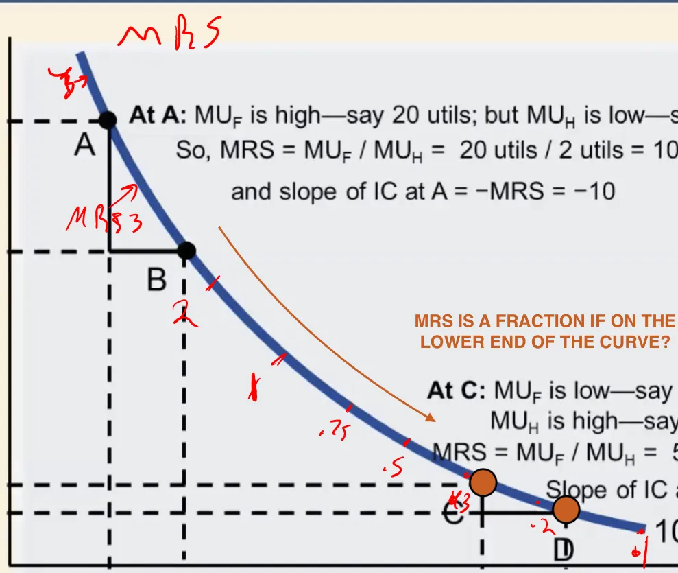
❔ Between the three graphs in the screenshot below, the consumer optimum varies even though the budget increased by the same amount. Would the only way to determine which of the IC curves is tangent be based on if the goods are normal or inferior (taste & preferences) for the individual consumer?

✔ If you know whether it’s normal or inferior, you can figure out which of the two graphs that he’s given you apply.

✏️ Which of the following graphs indicates that Minutes France is an inferior good? A. First Graph B. Second C. Neither D. Both

🕣
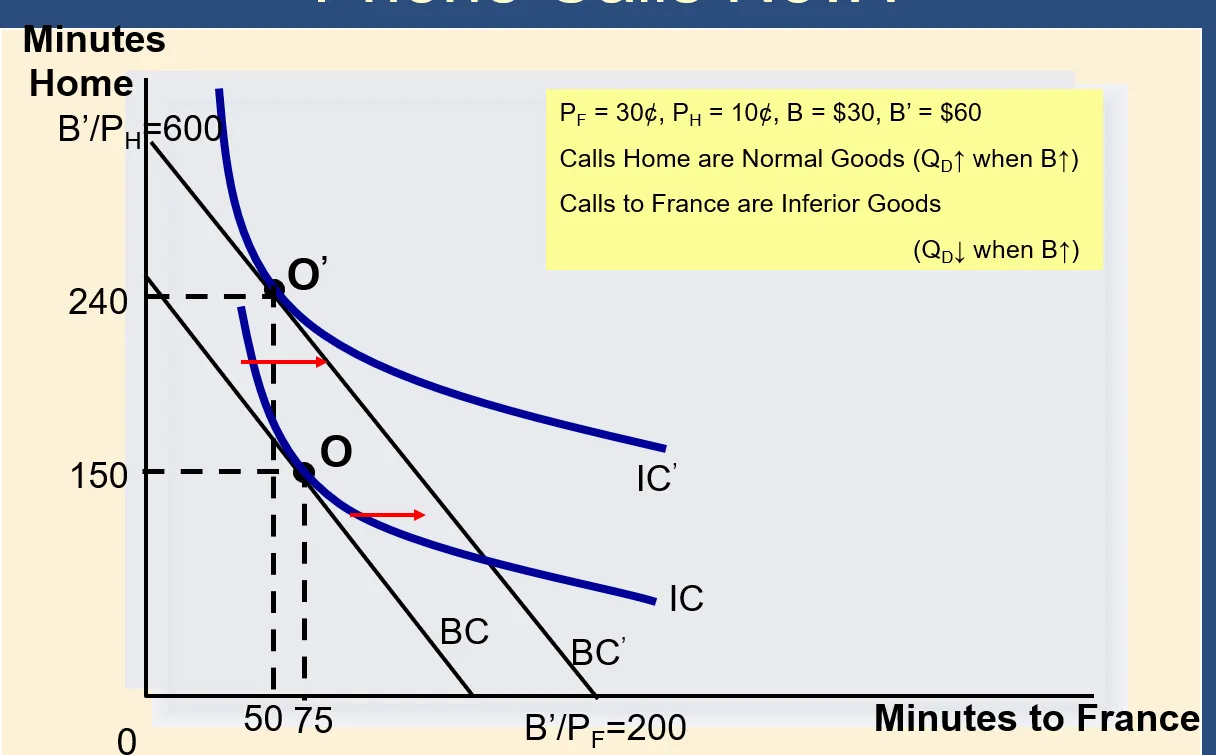
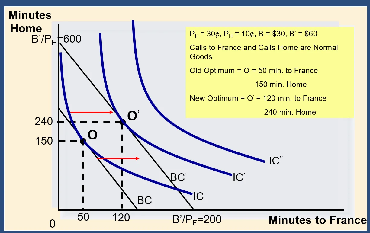
❔ So, other tangent IC curves exist, but they indicate other preferences than the ones of the consumer we are analyzing? Would we assume goods are normal when finding the consumer optimum in a problem if the good is not specified as normal or inferior?

✔ It’s true that every single person has different indifference curves. The indifference curves represent their preferences. Different people have different preferences, and so they have different indifference curves and they’ll have different tangent points and different choices.

Whenever you analyze a specific person, there will be specific indifference curves and there will be a specific consumer optimum. There will only be one for each person. That’s it. Just one, but if you look at a different person, they might have different indifference curves, different tangent points, and therefore different optimums.

Your second point, I think, is more important. You should never, unless we really, really hint strongly about something you never want to assume whether something is normal or inferior. If you’re wondering if a given good is normal or inferior, unless we tell you that it’s normal or inferior, you shouldn’t assume.

🕣 8:55pm
❔ I wanted to ask if those practice tests in Pearson (studyprep) are useful in preparing for the actual exam?

Are the questions on the real test similar in wording and structure to the practice questions, or are they quite different in style?

✔ The practice tests in Pearson’s can potentially be useful in preparing for the exam, but they’re going to include lots of material that we haven’t covered in lecture and therefore you don’t need to learn and won’t be on the exam. You’ll have to know the material well enough to be able to estimate whether something is going to be on the exam or not. Whether Bruce is covered in So you can look at the questions in the book and know which ones to ignore.

The best indications of what questions on the real test are going to be like are the short multiple choice questions in the problem sets. Those are the best indications, so let’s go look at a couple of those. I think that can be helpful and reassuring to help you calibrate.

Rob is a grad student at BU, but he likes to go to NYC. He occasionally takes the bus and occasionally takes the Acela. The price of bus trips rises and he takes fewer bus trips. Busses are an inferior good for Rob.

A. IE and SE are both ↑ B. IE and SE are both ↓ C. IE ↑ and SE ↓, IE > SE D. IE ↓ and SE ↑, IE > SE E. IE ↓ and SE ↑, IE < SE C. IE ↑ and SE ↓, IE < SE

Pbus↑, and I take fewer bus trips. Busses = inferior. SE: ↓ (more expensive) IE: poorer+inferior = ↑ CE: IE↑ > SE↓ : IE↑ → CE↑
IE↑ < SE↓ : SE↓ → CE↓ We are on line B, so IE↑ < SE↓

Feedback? Email munger.e1010@gmail.com 📧. Be sure to mention the page you are responding to.