👨🏫 Notes on Lecture 9
Pindyck and Rubinfeld: Section 4.4
Sections 9.1 – 9.4
Section 11.1
CS, PS, GS, SS…
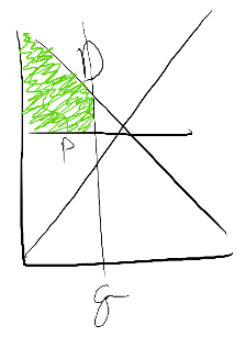
Section titled “CS, PS, GS, SS…”Consumer Surplus (CS) is all area:
Section titled “Consumer Surplus (CS) is all area:”- Under the demand curve
- Above the Price consumer pay
- To the left of the maximum number of units consumers actually consume.
Here is an illustration:
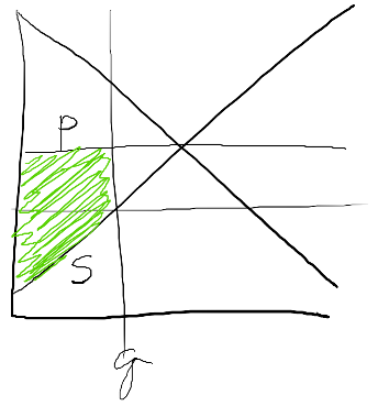
Producer Surplus (PS) is all area:
Section titled “Producer Surplus (PS) is all area:”- Above the Supply Curve
- Below the price producers receive
- To the left of the number of units actually produced.
Here is an illustration:
Government Surplus (GS) is either
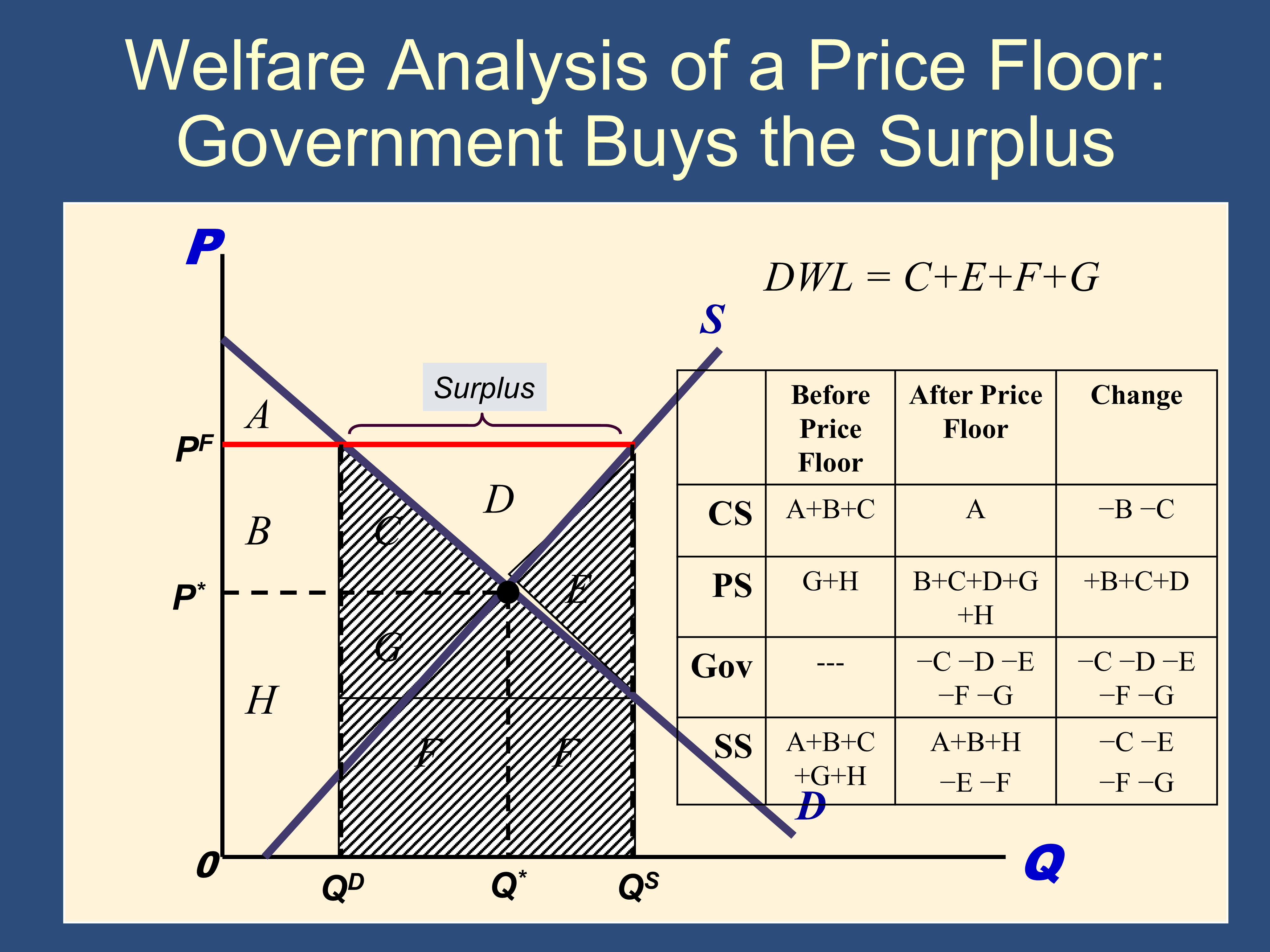
Section titled “Government Surplus (GS) is either” [Price Floor - gov’t buys surplus]
or
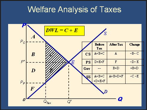
[Tax]
Social Surplus = Total Surplus
Section titled “Social Surplus = Total Surplus”
Practice problems
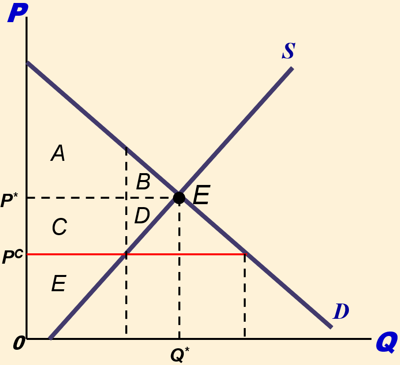
Section titled “Practice problems”✏ Fill in the following table for a binding price ceiling. Also identify the quantity demanded, quantity supplied, and the shortage or surplus, if any. What is the deadweight loss of the price floor?
| Before Price Ceiling | After Price Ceiling | Change | |
|---|---|---|---|
| CS | |||
| PS | |||
| SS |
✔ Click here to view answer
Solution is at the bottom of the page. ✅
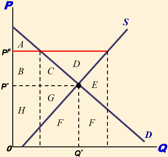
✏️ Fill in the following table for a binding price floor. The government does not buy the surplus. Also identify the quantity demanded, quantity supplied, and the amount of surplus produced, if any. What is the deadweight loss of the price floor?
| Before Price Floor | After Price Floor | Change | |
|---|---|---|---|
| CS | |||
| PS | |||
| SS |
✔ Click here to view answer
Solution is at the bottom of the page. ✅
✏️ Fill in the following table for a binding price floor. The government buys the surplus. Also identify the quantity demanded, quantity supplied, and the amount of surplus produced, if any. What is the deadweight loss of the price floor?
| Before Price Floor | After Price Floor | Change | |
|---|---|---|---|
| CS | |||
| PS | |||
| Gov | |||
| SS |
✔ Click here to view answer
Solution is at the bottom of the page. ✅
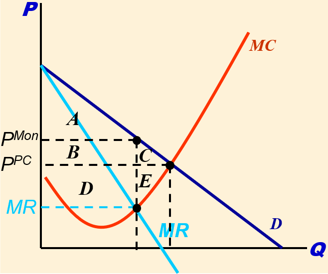
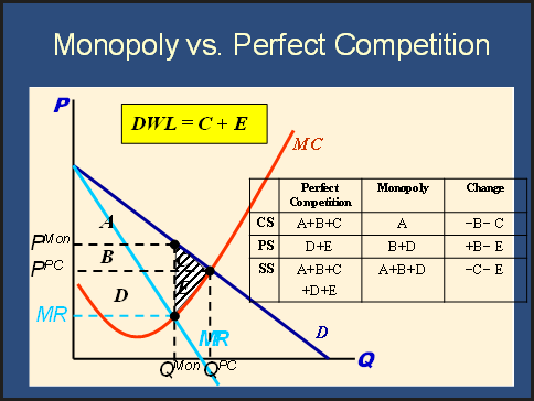
✏️ Fill in the following table describing the social welfare effects of Monopoly vs Perfect Competition. Also identify amount supplied by the monopoly and under perfect competition. What is the deadweight loss of the monopoly?
| Perfect Competition | Monopoly | Change | |
|---|---|---|---|
| CS | |||
| PS | |||
| SS |
✔ Click here to view answer
Solution is at the bottom of the page. ✅
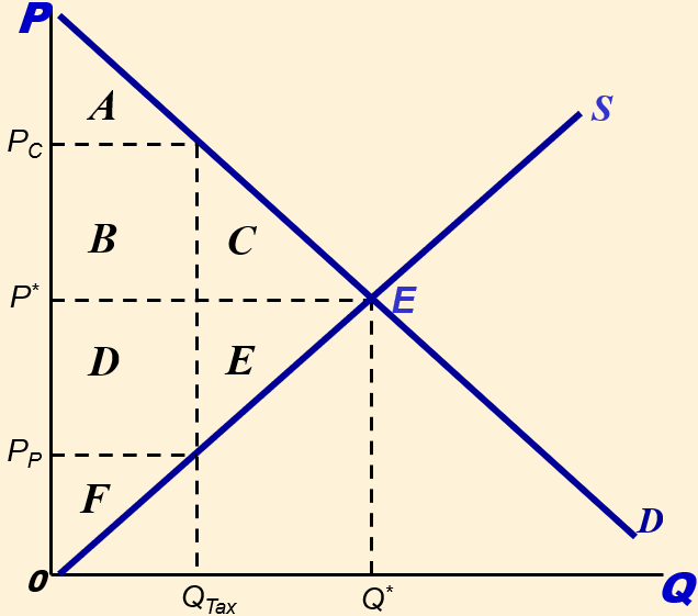
✏️ Fill in the following table describing the social welfare effects of a tax. What is the deadweight loss of the tax?
| Before Tax | After Tax | Change | |
|---|---|---|---|
| CS | |||
| PS | |||
| Gov | |||
| SS |
✔ Click here to view answer
Solution is at the bottom of the page. ✅
Solutions to the Exercises
Section titled “Solutions to the Exercises”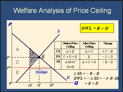
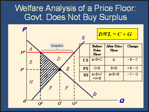
Binding vs. Non-binding Price Controls:
| Binding | Non-binding | |
|---|---|---|
| Price Floor | Binding Price Floor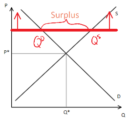 Price Floor > ⇨ Surplus | Non-binding Price Floor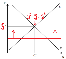 Price Floor < ⇨ NO EFFECT |
| Price Ceiling | Binding Price Ceiling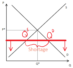 Price Ceiling < ⇨ Shortage | Non-binding Price Ceiling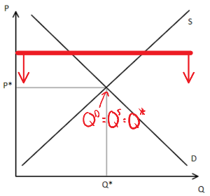 Price Ceiling > ⇨ NO EFFECT |
Feedback? Email munger.e1010@gmail.com 📧. Be sure to mention the page you are responding to.