🙋 Student Q&A (Review Week)

Click here to learn about timestamps and my process for answering questions. Section agendas can be found here. Email office hour questions to munger.e1010@gmail.com. PS1Q2=“Question 2 of Problem Set 1”

📅 Questions covered Mon, May 5 (Review Sess)

🕣
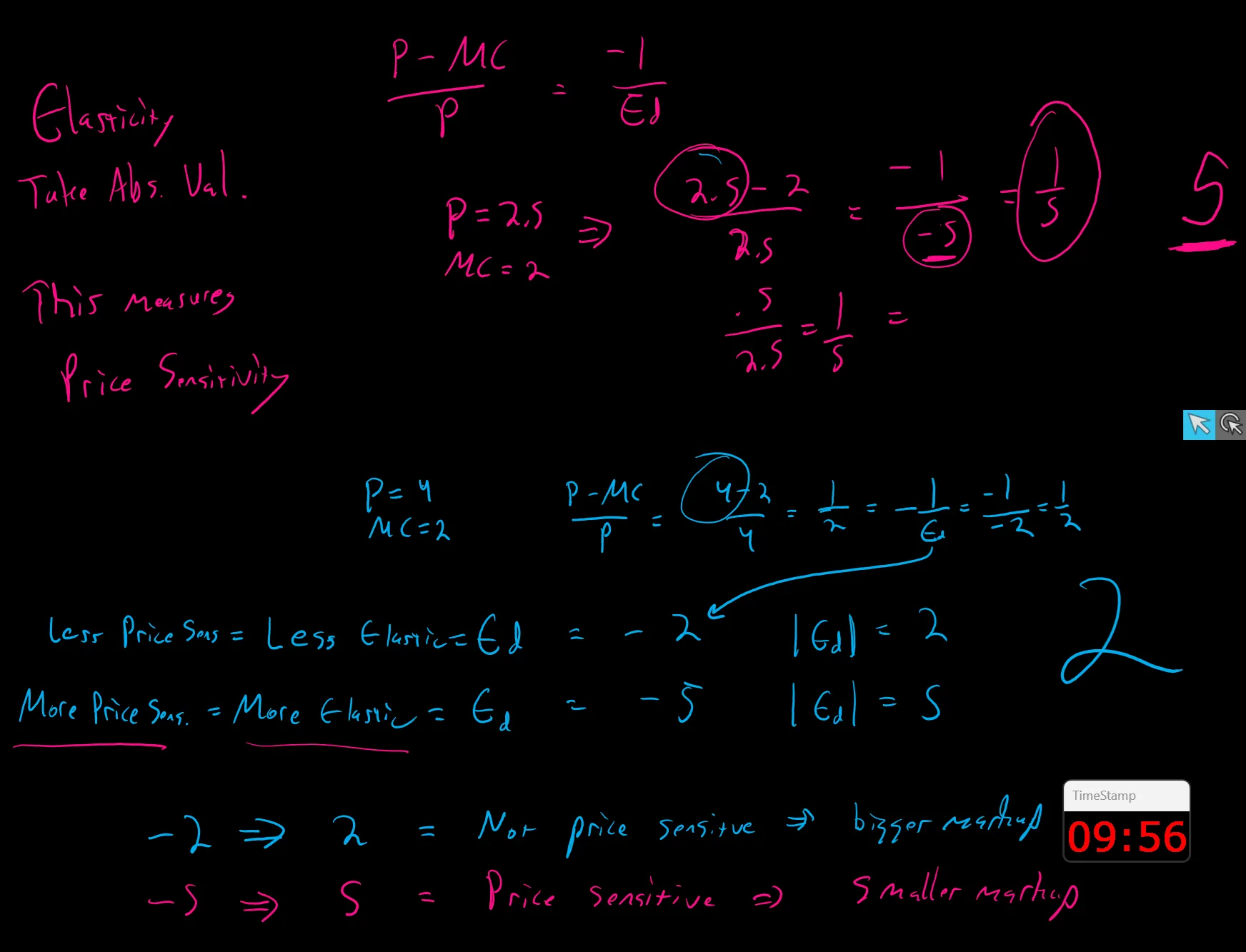
❔ Elasticity and the Price-cost markup (ie the Lerner Index)

✔

📅 Questions covered Thursday, May 7

🕣 8:58pm
❔ Can you explain problem set 10 question 5 on why option D is not correct? Thank you!

✔

🕣 Near start of session
❔ I hope this mail finds you well. I am reaching out to request whether you can do a full review of Problem Set 10 on Thursday. I did extremely poorly on this one despite feeling very confident about it. Clearly, I may have read too deeply into a question or not understood the material or concepts.

I would greatly appreciate if you can go over this one in depth.

✔ Done!

🕣 8:59pm
❔ Here are my questions for tonight’s section meeting.

HW3 Q17, Q19 HW5 Q6, HW6 Q3, HW7 Q4 and Q8

✔ See video HW3 Q17,

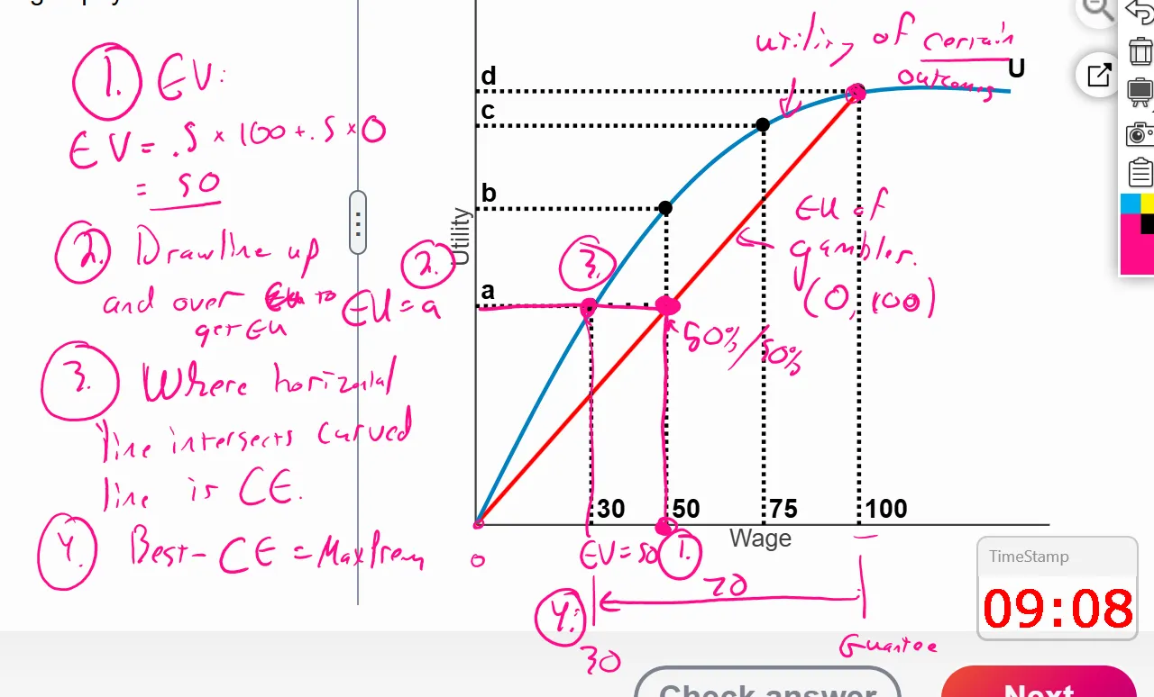
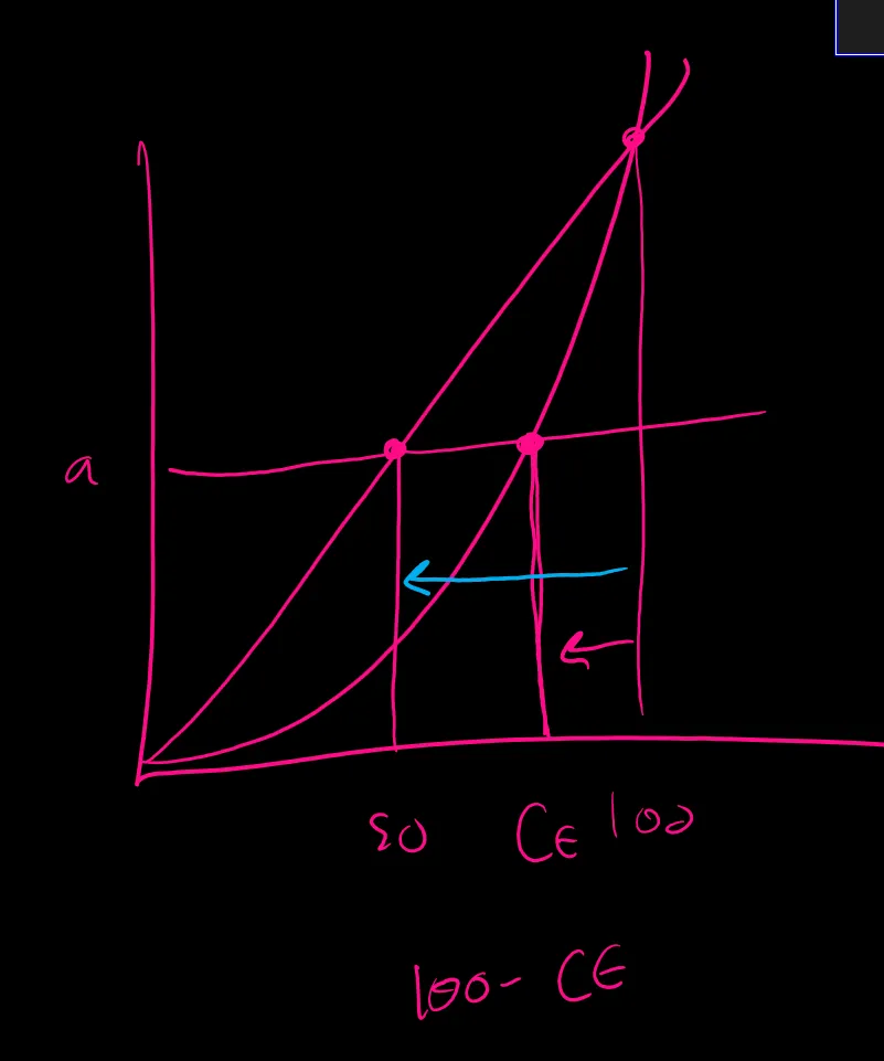
Fixed costs: https://1010.robmunger.com/l5/5notes/#identifying-fixed-and-variable-cost-from-a-formula

🕣 9:33pm
❔ I wouldn’t mind walking through the following if there is time:

Perfect competition problem Monopolistic problem The family of cost curves overview/reminder and maybe some questions related to what the curves tell us and what info they give us to solve problems.

Thank you for a great semester!!!

Fun fact: I got to use oligopoly and strategic interdependence in a conversation the other day! 🙂

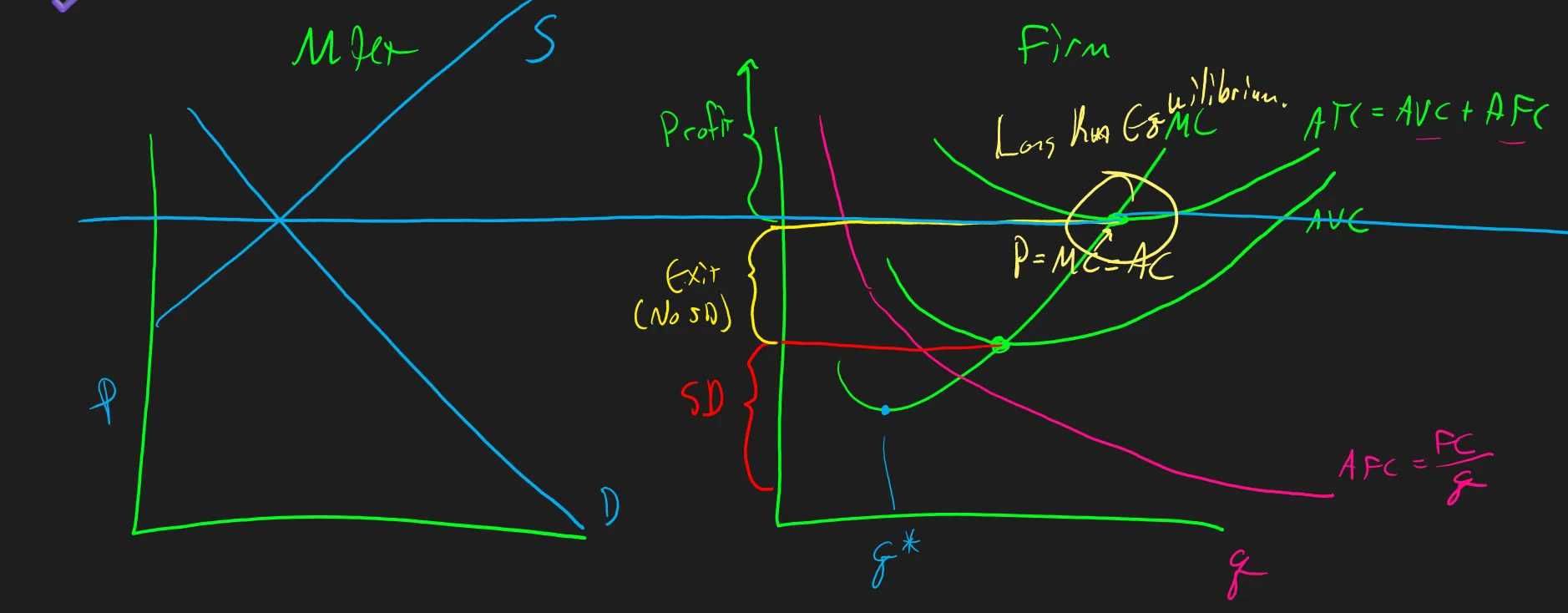
✔ See video. ✏️Perfect Comp

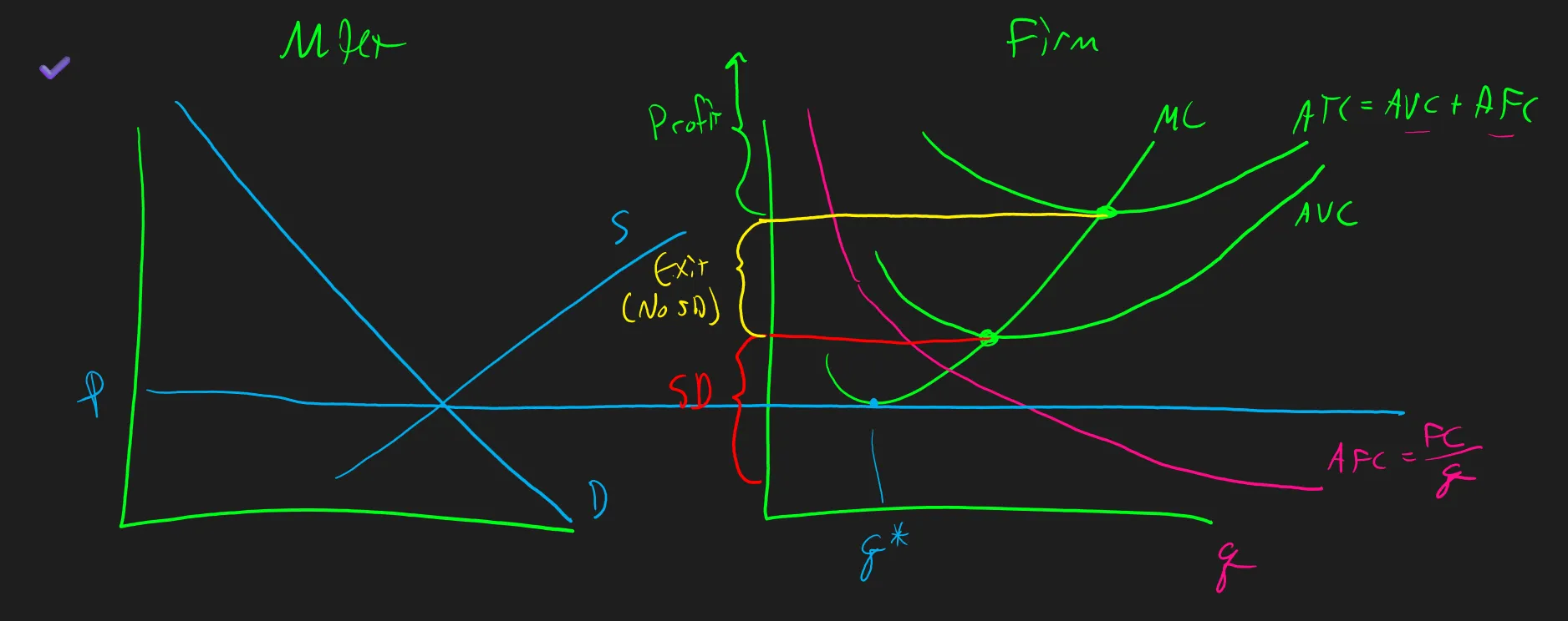
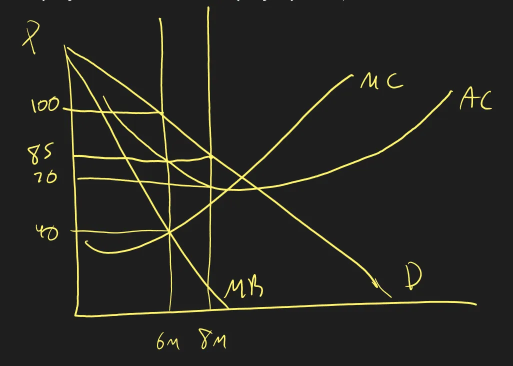
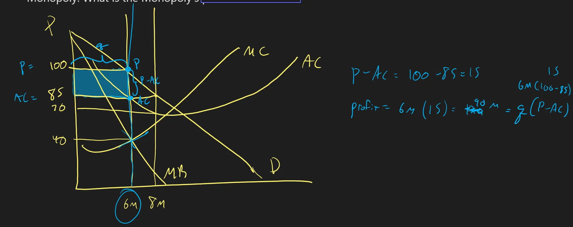
Monopoly. What is the Monopoly’s profit?

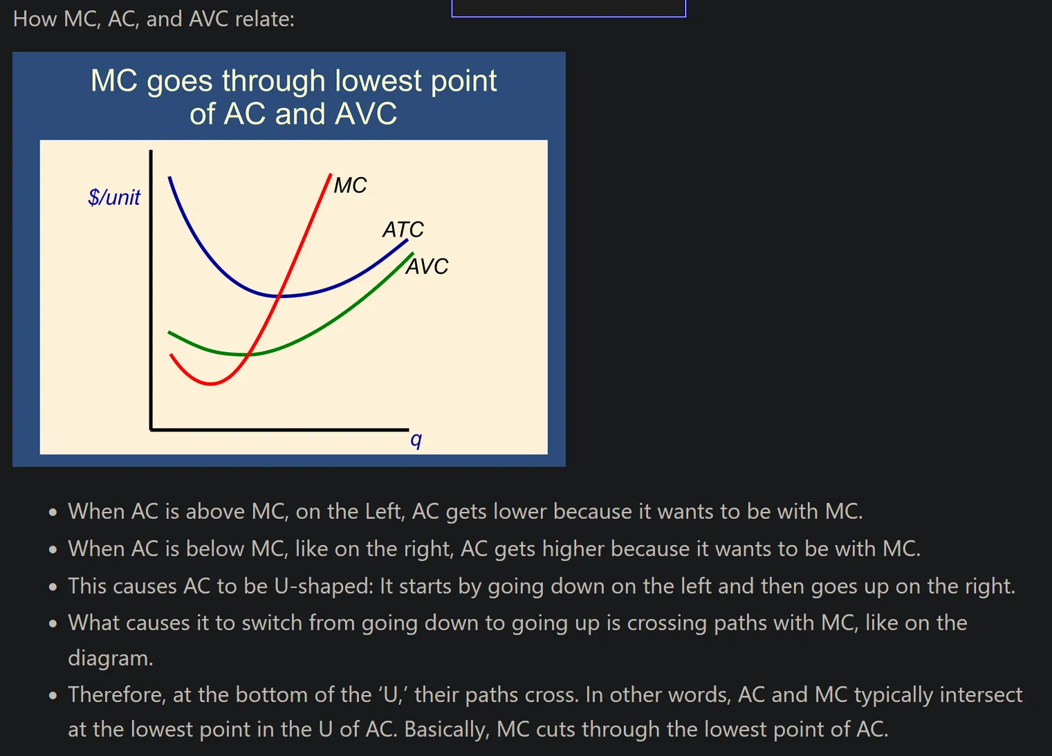
The family of cost curves overview/reminder and maybe some questions related to what the curves tell us and what info they give us to solve problems.

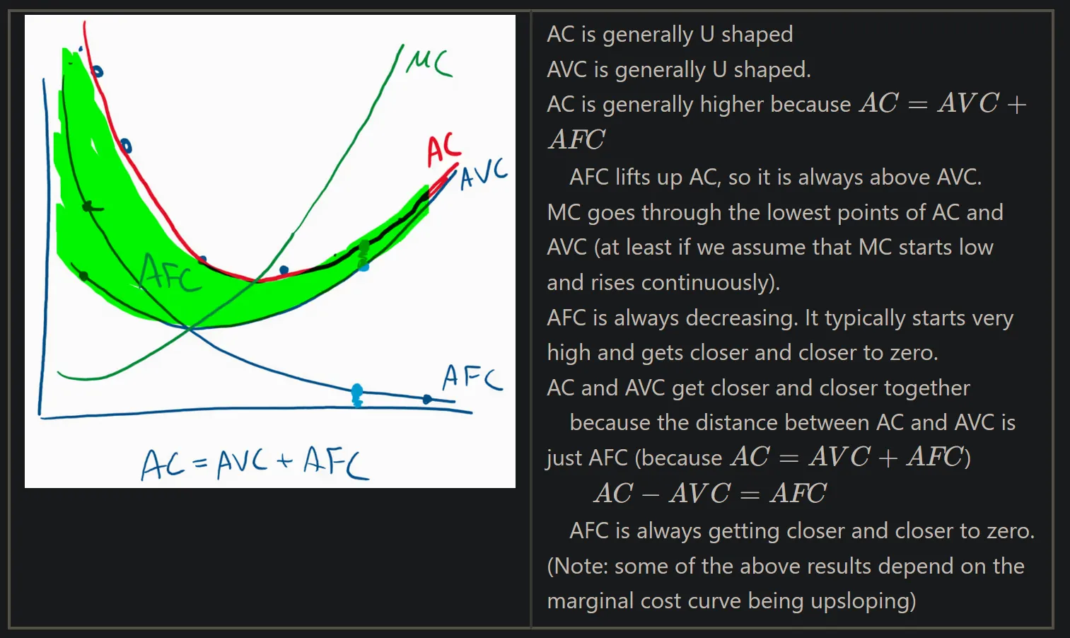
🕣 9:56pm
❔ If Canvas continues to remain unavailable during the time period for our final exam, how should we proceed?

✔ Bruce and I are monitoring the situation. The most important thing is just to keep studying. You may have to shift to other study resources, but the key study resources will always be the slides and redoing the problem sets. The textbook and my site are also always available and can be helpful.

https://dcegather.canvas.harvard.edu/courses/166274

📅 Questions covered Sunday, May 10

🕣 7:40pm
❔ Multiple NE.

Just finding it enough?

✔ Yes, identifying that there are multiple Nash equilibria and saying what they are is all we can do with our current tools. So far, we have two solution concepts:

1. A solution concept is a set of rules that, given a game, makes some sort of prediction.
2. The most famous solution concept we have is Nash Equilibrium. It is only a partial solution concept because sometimes there are no Nash equilibria, and sometimes there are lots of Nash equilibria. If you apply the Nash Equilibrium solution concept to a game, it will tell you which outcomes are possible and which seem reasonable according to the concept. It may give you one, multiple, or none.

That is where the concept stops, so that is all you can do. Just finding it is enough. Sometimes you can apply another solution concept. Our second solution concept is dominant strategy equilibrium. If all players have a dominant strategy, dominant strategy equilibrium predicts that strategy will happen. With a dominant strategy equilibrium, there are going to be fewer dominant strategy equilibria on average than there will be Nash equilibria. Sometimes you can cut down the set of possible outcomes by looking at dominant strategy equilibria or some other solution concept, but we have really only covered those two. I would expect a question to say, “Find the Nash equilibrium” or “Find the dominant strategies.”

🕣 7:42pm
❔ Insurance from the perspective of the insurance company

✔ From the insurance company’s perspective, you only need to worry about the payout to the customer. For example, if someone is guaranteed an income of $100,000 and there is a 20$40,000, the insurance company would need to pay $40,000 to make them whole.

That is the main concept: you have to pay out enough to make the customer whole. We are not saying that is the only way to run an insurance company. Those are just the examples that come up in this class, so if that is what you are looking at, you are good to go.

We will also care about how much it will cost to be an insurance company. When you are planning what to do as the insurance company, you do not know whether the person will get sick or not get sick. What you typically do is calculate the expected value of the payout. For example, suppose someone has an income of $100,000 and a potential loss of$40,000, and the chance of loss is 20%. You would calculate the expected value of the payout.

EV = 80% ×$0 + 20% × $40,000 = $8,000

Based on this calculation, the company expects their average payout to be $8,000. Note that there is no chance they will pay out$8,000 for a single customer. In practice, they will either pay out $0 or$40,000. For planning purposes, especially when you have many customers, it is smart to assume you will pay $8,000 for this customer. We often use expected value to get a sense of what they will pay out on average.

Suppose the premium is $10,000.

Customer: Customer has a guaranteed payout of $100,000 - \10,000 = $90,000. There is an 20% chance that they will lose $40,000 and be recompensated and an 80% chance that they won’t lose anything at all. Before we take into account the premium, therefore, they are guaranteed to have their starting income of $100,000. After we take into account the premium, then they are guaranteed to have a remaining income of $90,000 as per the calculation above.

Insurance Company: We can calcuate their profitability using the expected value. 20%: revenue = 10k, costs=40k. profit=10k-40k=-30k. 80%: revenue = 10k, costs=0. profit=10k-0=10k. Profit on average = EV = 20%×(-30K) + 80%×10K = -6K+8K = $2K.

We can also calculate the profit more easily, by using the EV of costs from before: EV of profits = Revenue - EV of costs = $10,000 - $8,000 = $2,000

Also subtract off administrative costs!

🕣 7:55pm
❔ Productive and allocative efficiency

✔

• ==Productive efficiency== refers to producing items at the lowest possible cost, i.e. at minimum average cost (ie choose the quantity that minimizes AC)
• ==Allocative efficiency== refers to producing all goods up to the     point where the marginal benefit to consumers is just equal to     the marginal cost to firms. ie in the market as a whole, MB = MC.

When we covered externalities, we focused on allocative efficiency. We were specifically talking about finding the allocatively efficient quantity of output in the market, in the presence of externalities.

Our intuition behind allocative efficiency was built up in the original “Omniscient Planner” slide.

• Efficiency is the property of a resource allocation of maximizing the total surplus received by all members of society.

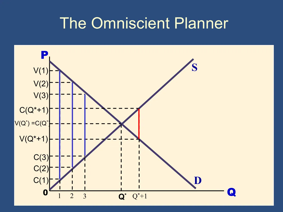
On the slide above, we are deciding how much we should produce as a society. The demand curve shows the value (or marginal benefit) to consumers of the good, which is determined by how much they are willing to pay. That means the demand curve sets the value. The page that explains this in detail is https://1010.robmunger.com/l9/stairstep/

The supply curve also shows the firm’s willingness to accept different prices for the good it is selling. That indirectly reveals its marginal costs, which in turn tells you the costs to society. https://1010.robmunger.com/l9/stairstep/ (at least in the absence of externalities).

When the value or marginal benefit is higher than the cost, we draw one of those blue lines. Producing and consuming the unit increases total social surplus in society, which is good and helps us move toward allocative efficiency. In contrast, once we get beyond a Q*, marginal benefit is lower than marginal cost. This lowers social surplus and therefore takes us farther away from economic efficiency. Allocative efficiency occurs at the sweet spot where we produce exactly Q*. At that point, we are producing exactly the right amount, and mb = mc.

If we assume the demand curve slopes downward and the supply curve slopes upward, all the good units should be produced to the left of Q*. All the blue lines will be to the left of Q*, and all the red lines will be to the right of Q*. When we reach Q*, the point where the demand curve intersects the supply curve, we maximize allocative efficiency. Since mb = mc at that point, it means we are producing where marginal benefit equals marginal cost. This should give some idea of why mb = mc is a good thing and why we call it allocative efficiency.

• ==Allocative efficiency== refers to producing all goods up to Q*, the point where the marginal benefit to consumers is just equal to the marginal cost to firms. ie in the market as a whole, MB = MC. This happens because at Q*, Demand equal supply, and demand tells you MB and supply tells you MC.

🕣 8:11pm
❔ hi Rob, for this question, inelastic supply curve, can you also tie it back to PS8, question 9?

✔

🕣 8:24pm
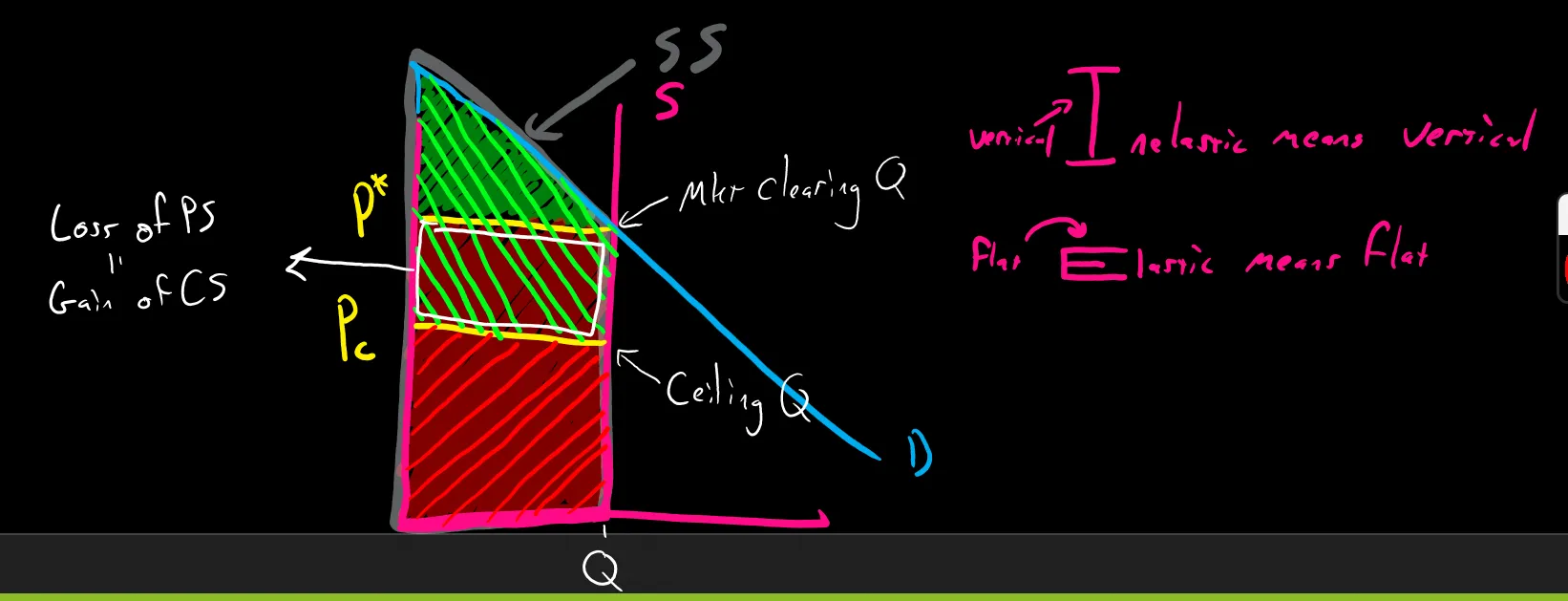
❔ Surplusses when supply curve is perfectly inelastic.

Question 1)

Could you go over how to solve this problem by the charts?

Suppose the supply curve is perfectly inelastic. If the gov imposes a price ceiling below the market clearing price, would a dead weight loss occur? ✔ See above

🕣
❔ While we’re at it, for CS and PS, Prof Watson went over this assuming the Demand curves are perfectly inelastic or perfectly elastic. But he didn’t go over if the supply curves are perfectly elastic or perfectly inelastic. Can we go over CS and PS under these circumstances?

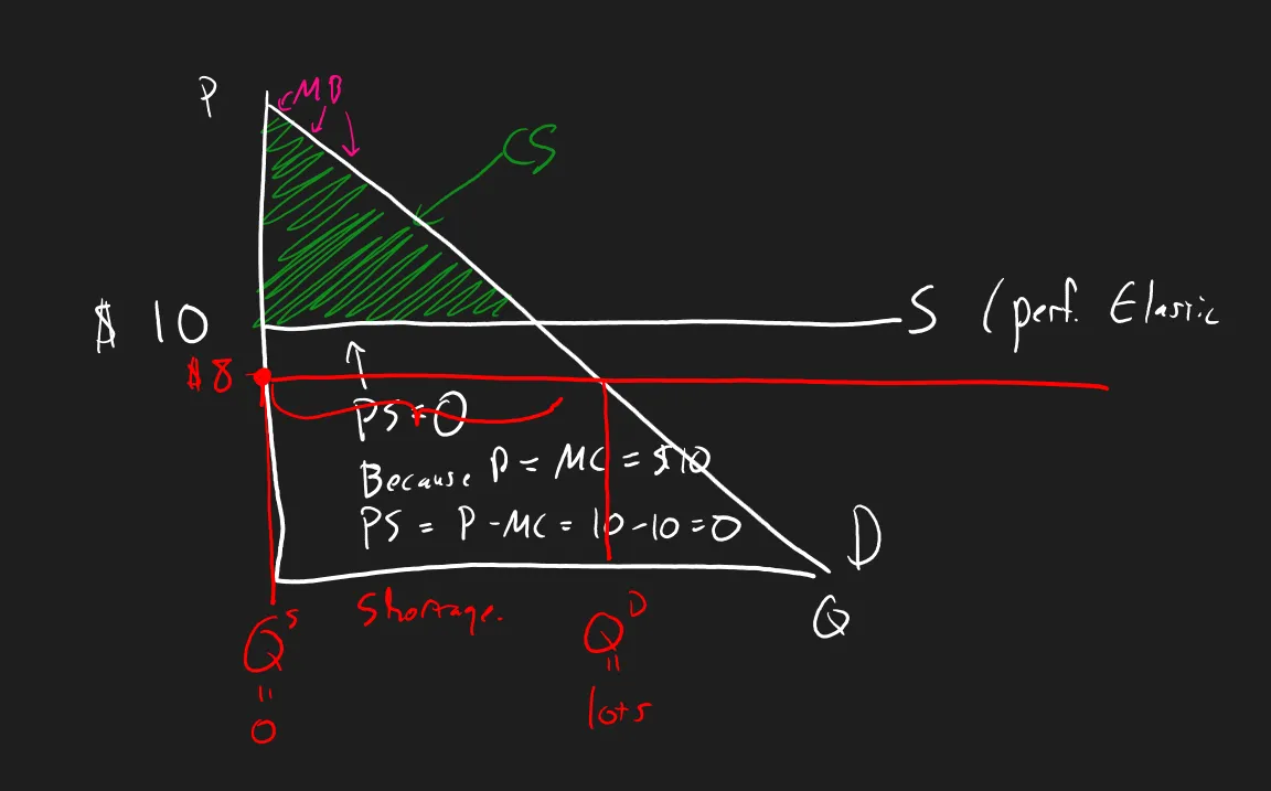
✔ We did this for perfectly inelastic supply curve, above. Below is perfectly elastic supply. Perfect elasticity means the firm is extremely price-sensitive. Elasticity always refers to price sensitivity, so perfect elasticity means perfect price sensitivity.

In the previous example, we had perfect inelasticity. That meant the firm would provide the same amount no matter what, and we found that was really good for social surplus. When the price ceiling was imposed, there was no shortage because the firm still provided the same amount, so there was no decrease in social surplus. I guess there was a shortage.

In the graph, firms are willing to supply zero units for $10 and a million units for$10. They’ll supply as much as you want for $10.

If the market price is $10.01, they’ll want to supply an infinite amount for$9.99. They won’t want to supply anything at all. For every unit supplied, the marginal cost is exactly $10, which leaves almost no room for producer surplus. If the market price is$10 (as it will be in this diagram), producer surplus for each firm is exactly zero because their price is $10 and their marginal cost is$10.

At any price below $10, there’ll be a complete shortage because no firm will want to produce anything. Before, social surplus was the same as consumer surplus because there was no producer surplus. Consumer surplus was consumer surplus.

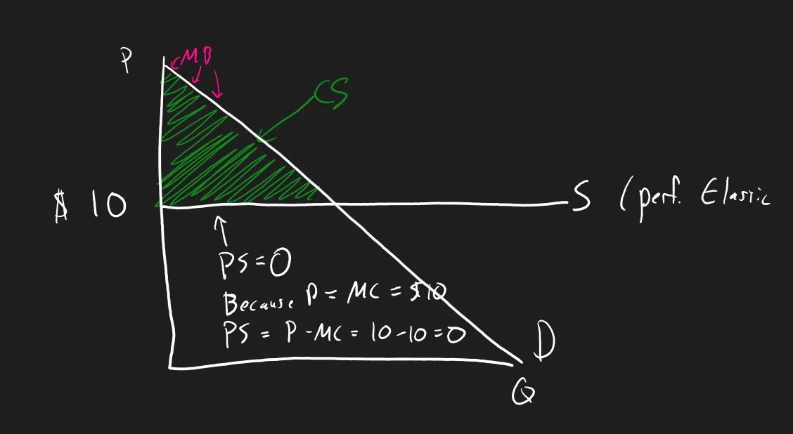
With the binding price ceiling, producers aren’t producing anything, so no one gets any surplus at all. The entire green triangle that used to be consumer surplus is gone and is now deadweight loss.

🕣 8:36pm
❔ Market Structure

✔ The default seems to be short run. If he doesn’t mention it’s long run or doesn’t give you an explicit clue that it’s long run, you’re usually safe assuming it’s short run.

🕣 8:47pm
❔ Repeated games

✔ see video.

🕣 8:55pm
❔ PS3 Q18
PS4 Q14
PS5 Q6, Q14
PS8-Q4, Q12

✔

🕣 9:17pm
❔ What is allocative efficiency, what kind of questions can be asked on it?

✔ Covered earlier and referenced several times throughout the recording.

🕣 9:18pm
❔ Could you please go through explain elasticity of Demand- How to use -1/Ed?

✔

✏️ Suppose the price elasticity of demand is -3. Is this elastic of inelastic?

✔|Ed| = absolute value of elasticity = 3 >1 elastic.

✏️ Suppose the price elasticity of demand is -3. What is the Lerner Index in this situation?

✔

$$\frac{P-MC}{P} = - \frac{1}{E_d}$$

The quantity on the left side of the equation above is the Lerner Index, also sometimes referred to as the price-cost markup. To calculate the Lerner Index, we only need to calculate the quantity on the right side of the equation: -1 / the price elasticity of demand. This is -1/(-3) = 1/3.

✏️ Suppose the Lerner Index is 1/3 and the MC =2. What is price?

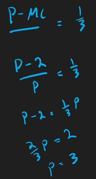
Now let’s review the Lerner index. The price is P=$3. The MC=$2. The markup of price above MC is $1. That markup is 1/3 of the price. Therefore, the Lerner index is 1/3.

$$\frac{P-MC}{P}$$

🕣
❔ Understanding that the final is cumulative, historically has their been a fairly even split between pre mid term and post mid term materials, or does it tend to weigh more heavily toward the material covered more recently. Trying to ensure I’m using my time most wisely, particularly in light of the canvas outage yesterday.

✔ It tends to favor post midterm questions. Perhaps a 70-30 or 60-40 split.